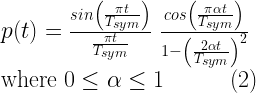
As mentioned earlier, the shortcomings of the sinc pulse can be addressed by making the transition band in the frequency domain less abrupt. The raised-cosine (RC) pulse comes with an adjustable transition band roll-off parameter  , using which the transition band’s rate of decay can be controlled. The RC pulse shaping function is expressed in frequency domain as

Correspondingly, in time domain, the impulse response is given by
This article is part of the book Wireless Communication Systems in Matlab, ISBN: 978-1720114352 available in ebook (PDF) format (click here) and Paperback (hardcopy) format (click here).
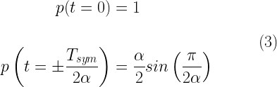
A simple evaluation of the equation (2) produces singularities (undefined points) at  and
and 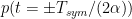 . The value of the raised-cosine pulse at these singularities can be obtained by applying L’Hospital’s rule [1] and the values are

The following Matlab codes generate a raised cosine pulse for the given symbol duration  and plot the time-domain view and the frequency response (shown in Figure 1). The RC pulse falls off at the rate of
  as
as  , which is a significant improvement when compared to the decay rate of sinc pulse which is
  . It satisfies Nyquist criterion for zero ISI – the pulse hits zero crossings at desired sampling instants. By controlling , the transition band roll-off in the frequency domain can be made gradual.
Program 1: raisedCosineFunction.m: Function for generating raised-cosine pulse(click here)
Program 2: test_RCPulse.m: Raised-cosine pulses and their manifestation in frequency domain
Tsym=1; %Symbol duration in seconds
L=10; % oversampling rate, each symbol contains L samples
Nsym = 80; %filter span in symbol durations
alphas=[0 0.3 0.5 1];%RC roll-off factors - valid range 0 to 1
Fs=L/Tsym;%sampling frequency
lineColors=['b','r','g','k','c']; i=1;legendString=cell(1,4);

for alpha=alphas %loop for various alpha values
	[rcPulse,t]=raisedCosineFunction(alpha,L,Nsym); %RC Pulse

	subplot(1,2,1); t=Tsym*t; %translate time base for given duration
	plot(t,rcPulse,lineColors(i));hold on; %plot time domain view
	[vals,f]=freqDomainView(rcPulse,Fs,'double');%See Chapter 1

	subplot(1,2,2);
	plot(f,abs(vals)/abs(vals(length(vals)/2+1)),lineColors(i));
	hold on;legendString{i}=strcat('\alpha =',num2str(alpha) );i=i+1;
end
subplot(1,2,1);title('Raised Cosine pulse'); legend(legendString);
subplot(1,2,2);title('Frequency response');legend(legendString);
References
[1] Clay S. Turner, Raised cosine and root raised cosine formulae, Wireless Systems Engineering, Inc, May 29, 2007.
Rate this post: 
 (16 votes, average: 3.19 out of 5)
Books by the author
 Wireless Communication Systems in Matlab Second Edition(PDF) Note: There is a rating embedded within this post, please visit this post to rate it. |  Digital Modulations using Python (PDF ebook) Note: There is a rating embedded within this post, please visit this post to rate it. |  Digital Modulations using Matlab (PDF ebook) Note: There is a rating embedded within this post, please visit this post to rate it. |
| Hand-picked Best books on Communication Engineering Best books on Signal Processing |
||
Topics in this chapter
| Pulse Shaping, Matched Filtering and Partial Response Signaling ● Introduction ● Nyquist Criterion for zero ISI ● Discrete-time model for a system with pulse shaping and matched filtering □ Rectangular pulse shaping □ Sinc pulse shaping □ Raised-cosine pulse shaping □ Square-root raised-cosine pulse shaping ● Eye Diagram ● Implementing a Matched Filter system with SRRC filtering □ Plotting the eye diagram □ Performance simulation ● Partial Response Signaling Models □ Impulse response and frequency response of PR signaling schemes ● Precoding □ Implementing a modulo-M precoder □ Simulation and results |
the matlab code is not working
Only a part of the code is given in this page. Full Matlab code is available only in the ebook.
If you are using the full code in the ebook and still encounter an error, please send error details (traceback) to the email address given in the preface of the book. Thanks
How does the raised cosine pulse help in reducing the effect of timing jitters at the receiver? Is it because of the reduced slope of side lobes of the pulse at zero crossing?
Timing jitter is present in any real system, which implies that the actual sampling instant at the receiver is not always optimal for every pulse.
A pulse shape can provide zero crossing at other pulse intervals, but a slight timing jitter can cause the sampling instant to move from the optimal sampling point.
Faster the pulse decays outside the pulse interval, lesser will be the impact of timing jitters on sampling of adjacent pulses.
Raised cosine filter’s roll-off factor provides a way to trade off between the data rate and the suppression of tail outside the pulse interval.