Key focus: Derive the Cramer-Rao lower bound for phase estimation applied to DSB transmission. Find out if an efficient estimator actually exists for phase estimation.
Problem formulation
Consider the DSB carrier frequency estimation problem given in the introductory chapter to estimation theory. A message is sent across a channel modulated by a sinusoidal carrier with carrier frequency = fc and amplitude= A. The transmitted signal gets affected by zero-mean AWGN noise when it travels across the medium. The receiver receives the signal and digitizes it for further processing.
To recover the message at the receiver, one has to know every details of the sinusoid:
1) Amplitude-A
2) Carrier Frequency – fc
3) Any uncertainty in its phase – ϕc.
Given a set of digitized samples x[n] and assuming that both amplitude and carrier frequency are known, we are tasked with the objective of estimating the phase of the embedded sinusoid (cosine wave). For analyzing this scenario we should have a model to begin with.
The digitized samples at the receiver are modeled as
![x[n] = A cos \left(2 \pi f_c n+ \phi_c \right) + w[n] ,\quad n=0,1,\cdots,N-1](https://s0.wp.com/latex.php?latex=x%5Bn%5D+%3D+A+cos+%5Cleft%282+%5Cpi+f_c+n%2B+%5Cphi_c+%5Cright%29+%2B+w%5Bn%5D+%2C%5Cquad+n%3D0%2C1%2C%5Ccdots%2CN-1&bg=ffffff&fg=000&s=1&c=20201002)
Here A and fc are assumed to be known and w[n] is an AWGN noise with mean μ=0 and variance=σ2. We will use CRLB and try to find an efficient estimator to estimate the phase component.
CRLB for Phase Estimation:
As a pre-requisite to this article, readers are advised to go through the previous article on “Steps to find CRLB”
In order to derive CRLB, we need to have a PDF (Probability Density Function) to begin with. Since the underlying noise is modeled as an AWGN noise with mean μ=0 and variance=σ2, the PDF of the observed sample that gets affected by this noise is given by a multivariate Gaussian distribution function.
![\begin{aligned} p(\mathbf{x} ; \phi) &= \prod_{n-0}^{N-1} \frac{1}{\sqrt{2 \pi \sigma^2}} exp \left[ -\frac{\left( \mathbf{x} - \mu_x \right)^2}{2 \sigma^2} \right] \\ &= \prod_{n-0}^{N-1} \frac{1}{\sqrt{2 \pi \sigma^2}} exp \left[ -\frac{\left( x[n] - \mu_x \right)^2}{2 \sigma^2} \right] \\ &= \frac{1}{\left( 2 \pi \sigma^2 \right)^{\frac{N}{2}}} exp \left[ - \frac{1}{2 \sigma^2} \sum_{n=0}^{N-1} \left( x[n] - \mu_x \right)^2 \right] \end{aligned}](https://s0.wp.com/latex.php?latex=%5Cbegin%7Baligned%7D+p%28%5Cmathbf%7Bx%7D+%3B+%5Cphi%29+%26%3D+%5Cprod_%7Bn-0%7D%5E%7BN-1%7D+%5Cfrac%7B1%7D%7B%5Csqrt%7B2+%5Cpi+%5Csigma%5E2%7D%7D+exp+%5Cleft%5B+-%5Cfrac%7B%5Cleft%28+%5Cmathbf%7Bx%7D+-+%5Cmu_x+%5Cright%29%5E2%7D%7B2+%5Csigma%5E2%7D+%5Cright%5D+%5C%5C+%26%3D+%5Cprod_%7Bn-0%7D%5E%7BN-1%7D+%5Cfrac%7B1%7D%7B%5Csqrt%7B2+%5Cpi+%5Csigma%5E2%7D%7D+exp+%5Cleft%5B+-%5Cfrac%7B%5Cleft%28+x%5Bn%5D+-+%5Cmu_x+%5Cright%29%5E2%7D%7B2+%5Csigma%5E2%7D+%5Cright%5D+%5C%5C+%26%3D++%5Cfrac%7B1%7D%7B%5Cleft%28+2+%5Cpi+%5Csigma%5E2+%5Cright%29%5E%7B%5Cfrac%7BN%7D%7B2%7D%7D%7D+exp+%5Cleft%5B+-+%5Cfrac%7B1%7D%7B2+%5Csigma%5E2%7D+%5Csum_%7Bn%3D0%7D%5E%7BN-1%7D+%5Cleft%28+x%5Bn%5D+-+%5Cmu_x+%5Cright%29%5E2+%5Cright%5D+%5Cend%7Baligned%7D+&bg=ffffff&fg=000&s=1&c=20201002)
The sample mean is given by
![\begin{aligned} \mu_x &= \frac{1}{N} \sum_{n=0}^{N-1} x[n] = \frac{1}{N} \sum_{n=0}^{N-1} \left[ A\;cos \left\{ 2 \pi f_c n + \phi_c \right\} + w[n] \right] \\ &= \frac{1}{N} \sum_{n=0}^{N-1} \left[ A\;cos \left\{ 2 \pi f_c n + \phi_c \right\} \right] + \frac{1}{N} \sum_{n=0}^{N-1} w[n] \\ &= \frac{1}{N} \sum_{n=0}^{N-1} \left[ A\;cos \left\{ 2 \pi f_c n + \phi_c \right\} \right] + 0 \\ &= \frac{1}{N} \sum_{n=0}^{N-1} \left[ A\;cos \left\{ 2 \pi f_c n + \phi_c \right\} \right] \end{aligned}](https://s0.wp.com/latex.php?latex=%5Cbegin%7Baligned%7D+%5Cmu_x+%26%3D++%5Cfrac%7B1%7D%7BN%7D+%5Csum_%7Bn%3D0%7D%5E%7BN-1%7D+x%5Bn%5D+%3D+%5Cfrac%7B1%7D%7BN%7D+%5Csum_%7Bn%3D0%7D%5E%7BN-1%7D+%5Cleft%5B+A%5C%3Bcos+%5Cleft%5C%7B+2+%5Cpi+f_c+n+%2B+%5Cphi_c+%5Cright%5C%7D+%2B+w%5Bn%5D+%5Cright%5D+%5C%5C+%26%3D+%5Cfrac%7B1%7D%7BN%7D+%5Csum_%7Bn%3D0%7D%5E%7BN-1%7D+%5Cleft%5B+A%5C%3Bcos+%5Cleft%5C%7B+2+%5Cpi+f_c+n+%2B+%5Cphi_c+%5Cright%5C%7D+%5Cright%5D+%2B+%5Cfrac%7B1%7D%7BN%7D+%5Csum_%7Bn%3D0%7D%5E%7BN-1%7D+w%5Bn%5D+%5C%5C+%26%3D+%5Cfrac%7B1%7D%7BN%7D+%5Csum_%7Bn%3D0%7D%5E%7BN-1%7D+%5Cleft%5B+A%5C%3Bcos+%5Cleft%5C%7B+2+%5Cpi+f_c+n+%2B+%5Cphi_c+%5Cright%5C%7D+%5Cright%5D+%2B+0+%5C%5C+%26%3D+%5Cfrac%7B1%7D%7BN%7D+%5Csum_%7Bn%3D0%7D%5E%7BN-1%7D+%5Cleft%5B+A%5C%3Bcos+%5Cleft%5C%7B+2+%5Cpi+f_c+n+%2B+%5Cphi_c+%5Cright%5C%7D+%5Cright%5D+%5Cend%7Baligned%7D+&bg=ffffff&fg=000&s=1&c=20201002)
The PDF is re-written as
![\displaystyle{ p(\mathbf{x}; \phi) = \frac{1}{\left( 2 \pi \sigma^2 \right)^{\frac{N}{2}}} exp \left[ -\frac{1}{2 \sigma^2} \sum_{n=0}^{N-1} \left[ x[n] - A cos\left( 2 \pi f_c n + \phi_c \right)\right]^2 \right]}](https://s0.wp.com/latex.php?latex=%5Cdisplaystyle%7B+p%28%5Cmathbf%7Bx%7D%3B+%5Cphi%29+%3D+%5Cfrac%7B1%7D%7B%5Cleft%28+2+%5Cpi+%5Csigma%5E2+%5Cright%29%5E%7B%5Cfrac%7BN%7D%7B2%7D%7D%7D+exp+%5Cleft%5B+-%5Cfrac%7B1%7D%7B2+%5Csigma%5E2%7D+%5Csum_%7Bn%3D0%7D%5E%7BN-1%7D+%5Cleft%5B+x%5Bn%5D+-+A+cos%5Cleft%28+2+%5Cpi+f_c+n+%2B+%5Cphi_c+%5Cright%29%5Cright%5D%5E2++%5Cright%5D%7D+&bg=ffffff&fg=000&s=1&c=20201002)
Since the observed samples x[n] are fixed in the above equation, we will use the likelihood notation instead of PDF notation. That is,  is simply rewritten in terms of log likelihood as
  . The log likelihood function is given by
![\displaystyle{ ln\; L(\mathbf{x;\phi }) = - \frac{N}{2} ln \left( 2 \pi \sigma^2\right) + \left[ - \frac{1}{2 \sigma^2} \sum_{n=0}^{N-1} \left( x[n] - A cos \left\{ 2 \pi f_c n + \phi_c \right\} \right)^2 \right] }](https://s0.wp.com/latex.php?latex=%5Cdisplaystyle%7B+ln%5C%3B+L%28%5Cmathbf%7Bx%3B%5Cphi+%7D%29+%3D+-+%5Cfrac%7BN%7D%7B2%7D+ln+%5Cleft%28+2+%5Cpi+%5Csigma%5E2%5Cright%29+%2B+%5Cleft%5B++-+%5Cfrac%7B1%7D%7B2+%5Csigma%5E2%7D+%5Csum_%7Bn%3D0%7D%5E%7BN-1%7D+%5Cleft%28+x%5Bn%5D+-+A+cos+%5Cleft%5C%7B+2+%5Cpi+f_c+n+%2B+%5Cphi_c+%5Cright%5C%7D+%5Cright%29%5E2+%5Cright%5D+%7D++&bg=ffffff&fg=000&s=1&c=20201002)
For simplicity,we will denote ϕc as ϕ. Next, take the first partial derivative of log likelihood function with respect to ϕ.
![\displaystyle{ \begin{aligned}\frac{\partial \; ln \; L( \mathbf{x;\phi})}{\partial \phi} &= -\frac{1}{\sigma^2} \sum_{n-0}^{N-1} \left[ x[n] - A cos \left( 2 \pi f_c n + \phi \right) \right] A sin \left( 2 \pi f_c n + \phi \right) \\ &=-\frac{A}{\sigma^2} \sum_{n-0}^{N-1} \left[ x[n] sin (2 \pi f_c n + \phi) - \frac{A}{2} sin( 4 \pi f_c n + 2 \phi) \right] \end{aligned}}](https://s0.wp.com/latex.php?latex=%5Cdisplaystyle%7B+%5Cbegin%7Baligned%7D%5Cfrac%7B%5Cpartial+%5C%3B+ln+%5C%3B+L%28+%5Cmathbf%7Bx%3B%5Cphi%7D%29%7D%7B%5Cpartial+%5Cphi%7D+%26%3D+-%5Cfrac%7B1%7D%7B%5Csigma%5E2%7D+%5Csum_%7Bn-0%7D%5E%7BN-1%7D+%5Cleft%5B+x%5Bn%5D+-+A+cos+%5Cleft%28+2+%5Cpi+f_c+n+%2B+%5Cphi+%5Cright%29+%5Cright%5D+A+sin+%5Cleft%28+2+%5Cpi+f_c+n+%2B+%5Cphi+%5Cright%29+%5C%5C+%26%3D-%5Cfrac%7BA%7D%7B%5Csigma%5E2%7D+%5Csum_%7Bn-0%7D%5E%7BN-1%7D+%5Cleft%5B+x%5Bn%5D+sin+%282+%5Cpi+f_c+n+%2B+%5Cphi%29+-+%5Cfrac%7BA%7D%7B2%7D+sin%28+4+%5Cpi+f_c+n+%2B+2+%5Cphi%29+%5Cright%5D+%5Cend%7Baligned%7D%7D+&bg=ffffff&fg=000&s=1&c=20201002)
Taking the second partial derivative of the log likelihood function,
![\displaystyle{ \frac{\partial^2 \; ln \; L( \mathbf{x;\phi})}{\partial^2 \phi} = -\frac{A}{\sigma^2} \sum_{n-0}^{N-1} \left[ x[n] cos (2 \pi f_c n + \phi) - A cos( 4 \pi f_c n + 2 \phi) \right] }](https://s0.wp.com/latex.php?latex=%5Cdisplaystyle%7B+%5Cfrac%7B%5Cpartial%5E2+%5C%3B+ln+%5C%3B+L%28+%5Cmathbf%7Bx%3B%5Cphi%7D%29%7D%7B%5Cpartial%5E2+%5Cphi%7D+%3D+-%5Cfrac%7BA%7D%7B%5Csigma%5E2%7D+%5Csum_%7Bn-0%7D%5E%7BN-1%7D+%5Cleft%5B+x%5Bn%5D+cos+%282+%5Cpi+f_c+n+%2B+%5Cphi%29+-+A+cos%28+4+%5Cpi+f_c+n+%2B+2+%5Cphi%29+%5Cright%5D+%7D+&bg=ffffff&fg=000&s=1&c=20201002)
Since the above term is still dependent on the observed samples \(x[n]\), take expectation of the entire equation to average out the variations.
![\displaystyle{\begin{aligned} -E \left[\frac{\partial^2 \; ln \; L(\mathbf{x;\phi})}{\partial^2 \phi} \right] &= \frac{A}{\sigma^2} \sum_{n=0}^{N-1} \left[ E(x[n])cos\left( 2 \pi f_c n + \phi \right) - A \; cos\left( 4 \pi f_c n + 2 \phi \right) \right] \\ &= \frac{A}{\sigma^2} \sum_{n=0}^{N-1} \left[ A \; cos^2 \left( 2 \pi f_c n + \phi \right) - A \; cos \left( 4 \pi f_c n + 2 \phi \right)\right] \\ &= \frac{A^2}{\sigma^2} \sum_{n=0}^{N-1} \left[ \frac{1}{2} + \frac{1}{2} cos \left( 4 \pi f_c n + 2 \phi \right) - cos\left( 4 \pi f_c n + 2 \phi \right) \right] \\ &=\frac{A^2}{2 \sigma^2} \sum_{n=0}^{N-1} \left[ 1 - cos \left( 4 \pi f_c n + 2 \phi\right)\right] \\ & \approx \frac{A^2}{2 \sigma^2} \left[ N - 0 \right] = \frac{N A^2}{2 \sigma^2}\end{aligned}}](https://s0.wp.com/latex.php?latex=%5Cdisplaystyle%7B%5Cbegin%7Baligned%7D+-E+%5Cleft%5B%5Cfrac%7B%5Cpartial%5E2+%5C%3B+ln+%5C%3B+L%28%5Cmathbf%7Bx%3B%5Cphi%7D%29%7D%7B%5Cpartial%5E2+%5Cphi%7D+%5Cright%5D+%26%3D+%5Cfrac%7BA%7D%7B%5Csigma%5E2%7D+%5Csum_%7Bn%3D0%7D%5E%7BN-1%7D+%5Cleft%5B+E%28x%5Bn%5D%29cos%5Cleft%28+2+%5Cpi+f_c+n+%2B+%5Cphi+%5Cright%29+-+A+%5C%3B+cos%5Cleft%28+4+%5Cpi+f_c+n+%2B+2+%5Cphi+%5Cright%29+%5Cright%5D+%5C%5C+%26%3D+%5Cfrac%7BA%7D%7B%5Csigma%5E2%7D+%5Csum_%7Bn%3D0%7D%5E%7BN-1%7D+%5Cleft%5B+A+%5C%3B+cos%5E2+%5Cleft%28+2+%5Cpi+f_c+n+%2B+%5Cphi+%5Cright%29+-+A+%5C%3B+cos+%5Cleft%28+4+%5Cpi+f_c+n+%2B+2+%5Cphi+%5Cright%29%5Cright%5D+%5C%5C+%26%3D+%5Cfrac%7BA%5E2%7D%7B%5Csigma%5E2%7D+%5Csum_%7Bn%3D0%7D%5E%7BN-1%7D+%5Cleft%5B+%5Cfrac%7B1%7D%7B2%7D+%2B+%5Cfrac%7B1%7D%7B2%7D+cos+%5Cleft%28+4+%5Cpi+f_c+n+%2B+2+%5Cphi+%5Cright%29+-+cos%5Cleft%28+4+%5Cpi+f_c+n+%2B+2+%5Cphi+%5Cright%29+%5Cright%5D+%5C%5C+%26%3D%5Cfrac%7BA%5E2%7D%7B2+%5Csigma%5E2%7D+%5Csum_%7Bn%3D0%7D%5E%7BN-1%7D+%5Cleft%5B+1+-+cos+%5Cleft%28+4+%5Cpi+f_c+n+%2B+2+%5Cphi%5Cright%29%5Cright%5D+%5C%5C+%26+%5Capprox+%5Cfrac%7BA%5E2%7D%7B2+%5Csigma%5E2%7D+%5Cleft%5B+N+-+0+%5Cright%5D+%3D+%5Cfrac%7BN+A%5E2%7D%7B2+%5Csigma%5E2%7D%5Cend%7Baligned%7D%7D++&bg=ffffff&fg=000&s=1&c=20201002)
Let’s derive the terms like fisher information, CRLB and find out whether we can find an efficient estimator from the equations.
Fisher Information:
The Fisher Information for the given problem is
![\displaystyle{ I(\phi) = -E \left[\frac{\partial^2 \; ln \; L(\mathbf{x;\phi})}{\partial^2 \phi} \right] = \frac{N A^2}{ 2 \sigma^2}}](https://s0.wp.com/latex.php?latex=%5Cdisplaystyle%7B+I%28%5Cphi%29+%3D+-E+%5Cleft%5B%5Cfrac%7B%5Cpartial%5E2+%5C%3B+ln+%5C%3B+L%28%5Cmathbf%7Bx%3B%5Cphi%7D%29%7D%7B%5Cpartial%5E2+%5Cphi%7D+%5Cright%5D+%3D+%5Cfrac%7BN+A%5E2%7D%7B+2+%5Csigma%5E2%7D%7D+&bg=ffffff&fg=000&s=1&c=20201002)
Cramer Rao Lower Bound:
The CRLB is the reciprocal of Fisher Information.

The variance of any estimator estimating the phase of the carrier for given problem will always be higher than this CRLB. That is,
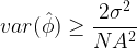
As we can see from the above result, that the variance of the estimates 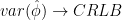 as
as  . Such estimators are called Asymptotically Efficient Estimators.

An efficient estimator exists if and only if the first partial derivative of log likelihood function can be written in the form
![\displaystyle{ \frac{\partial \; ln \; L(\mathbf{x;\phi}) }{\partial \phi} = I(\phi) \left[ g(\mathbf{x}) - \phi \right]}](https://s0.wp.com/latex.php?latex=%5Cdisplaystyle%7B+%5Cfrac%7B%5Cpartial+%5C%3B+ln+%5C%3B+L%28%5Cmathbf%7Bx%3B%5Cphi%7D%29+%7D%7B%5Cpartial+%5Cphi%7D+%3D+I%28%5Cphi%29+%5Cleft%5B+g%28%5Cmathbf%7Bx%7D%29+-+%5Cphi+%5Cright%5D%7D+&bg=ffffff&fg=000&s=1&c=20201002)
Re-writing our earlier result,
![\displaystyle{ \frac{\partial \; ln \; L(\mathbf{x;\phi}) }{\partial \phi} = - \frac{A}{\sigma^2} \sum_{n=0}^{N-1} \left[ x[n] \; sin \left( 2 \pi f_c n + \phi\right) - \frac{A}{2} sin \left( 4 \pi f_c n + 2 \phi \right) \right]}](https://s0.wp.com/latex.php?latex=%5Cdisplaystyle%7B+%5Cfrac%7B%5Cpartial+%5C%3B+ln+%5C%3B+L%28%5Cmathbf%7Bx%3B%5Cphi%7D%29+%7D%7B%5Cpartial+%5Cphi%7D+%3D+-+%5Cfrac%7BA%7D%7B%5Csigma%5E2%7D+%5Csum_%7Bn%3D0%7D%5E%7BN-1%7D+%5Cleft%5B+x%5Bn%5D+%5C%3B+sin+%5Cleft%28+2+%5Cpi+f_c+n+%2B+%5Cphi%5Cright%29+-+%5Cfrac%7BA%7D%7B2%7D+sin+%5Cleft%28+4+%5Cpi+f_c+n+%2B+2+%5Cphi+%5Cright%29+%5Cright%5D%7D+&bg=ffffff&fg=000&s=1&c=20201002)
We can clearly see that the above two equations are not having the same form. Thus, an efficient estimator does not exist for this problem.
Rate this article: 
 (6 votes, average: 4.33 out of 5)
For further reading
Related Topics
Books by the author
 Wireless Communication Systems in Matlab Second Edition(PDF)  (168 votes, average: 3.71 out of 5) (168 votes, average: 3.71 out of 5) |  Digital Modulations using Python (PDF ebook) (124 votes, average: 3.60 out of 5) |  Digital Modulations using Matlab (PDF ebook) (129 votes, average: 3.71 out of 5) |
| Hand-picked Best books on Communication Engineering Best books on Signal Processing |
||