Convolution operation is ubiquitous in signal processing applications. The mathematics of convolution is strongly rooted in operation on polynomials. The intent of this text is to enhance the understanding on mathematical details of convolution.
Polynomial functions:
Polynomial functions are expressions consisting of sum of terms, where each term includes one or more variables raised to a non-negative power and each term may be scaled by a coefficient. Addition, Subtraction and multiplication of polynomials are possible.
This article is part of the following books |
Polynomial functions can involve one or more variables. For example, following polynomial expression is a function of variable x. It involves sum of 3 terms where each term is scaled by a coefficient. Polynomial expression involving two variables ‘x’ and ‘y’ is given next.


Representing single variable polynomial functions:
Polynomial functions involving single variable is of specific interest here. In general a single variable (say ‘x’) polynomial is expressed in the following sum of terms form, where  are coefficients of the polynomial.

The degree or order of the polynomial function is the highest power of  with a non-zero coefficient. The above equation can be written as

It is also represented by a vector of coefficients as ![a=[a_0,a_1,a_2,...,a_{n-1}]](https://s0.wp.com/latex.php?latex=a%3D%5Ba_0%2Ca_1%2Ca_2%2C...%2Ca_%7Bn-1%7D%5D&bg=ffffff&fg=000&s=0&c=20201002) .
.
Polynomials can also be represented using their roots which is a product of linear terms form, as explained later.
Multiplication of polynomials and linear convolution:
As indicated earlier, mathematical operations like additions, subtractions and multiplications can be performed on polynomial functions. Addition or subtraction of polynomials is straight forward. Multiplication of polynomials is of specific interest in the context of subject discussed here.
Computing the product of two polynomials represented by the coefficient vectors ![a=[a_0,a_1,a_2,...,a_n]](https://s0.wp.com/latex.php?latex=a%3D%5Ba_0%2Ca_1%2Ca_2%2C...%2Ca_n%5D&bg=ffffff&fg=000&s=0&c=20201002) and
and ![b=[b_0,b_1,b_2,...,b_n]](https://s0.wp.com/latex.php?latex=b%3D%5Bb_0%2Cb_1%2Cb_2%2C...%2Cb_n%5D&bg=ffffff&fg=000&s=0&c=20201002) . The usual representation of such polynomials is given by
. The usual representation of such polynomials is given by


The product vector is represented as

Or equivalently as
![p(x) . q(x)=(p\ast q)(x)=a.b=[c_0,c_1,c_2,\cdots,c_{n+m}] \; , \;where](https://s0.wp.com/latex.php?latex=p%28x%29+.+q%28x%29%3D%28p%5Cast+q%29%28x%29%3Da.b%3D%5Bc_0%2Cc_1%2Cc_2%2C%5Ccdots%2Cc_%7Bn%2Bm%7D%5D+%5C%3B+%2C+%5C%3Bwhere+&bg=ffffff&fg=000&s=2&c=20201002)

Since the subscripts obey the equality  , changing the subscript
  to
to  gives
gives
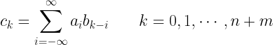
Which, when written in terms of indices, provides the most widely used form seen in signal processing text books.
![c[k]=\displaystyle{\sum_{i=-\infty}^{\infty}a[i]b[k-i]} \quad\quad k=0,1,\cdots,n+m](https://s0.wp.com/latex.php?latex=c%5Bk%5D%3D%5Cdisplaystyle%7B%5Csum_%7Bi%3D-%5Cinfty%7D%5E%7B%5Cinfty%7Da%5Bi%5Db%5Bk-i%5D%7D+%5Cquad%5Cquad+k%3D0%2C1%2C%5Ccdots%2Cn%2Bm+&bg=ffffff&fg=000&s=2&c=20201002)
This operation is referred as convolution (linear convolution, to be precise), denoted as  . It is very closely related to other operations on vectors – cross-correlation, auto-correlation and moving average computation.
Thus when we are computing convolution, we are actually multiplying two polynomials.
Note, that if the polynomials have  and
and  terms, their multiplication produces
  terms.
The straightforward algorithm (shown below) that implements the above product expression will consume  time. A better algorithm is a necessity. It turns out that viewing the polynomials as product of linear factors of complex roots will save much of the computations. This forms the basis for Fast Fourier Transform, where nth root of unity is utilized recursively to do the computation in frequency domain (in signal processing perspective). More about this later.
for i = 0:n+m,
   ci = 0;
for i = 0 :n,
   for k = 0 to m,
      c[i+k] = c[i+k] + a[i] · b[k];
Toeplitz Matrix and Convolution:
Convolution operation of two sequences can be viewed as multiplying two matrices as explained next. Given a LTI (Linear Time Invariant) system with impulse response ![h[n]](https://s0.wp.com/latex.php?latex=h%5Bn%5D&bg=ffffff&fg=000&s=0&c=20201002) and an input sequence
and an input sequence ![x[n]](https://s0.wp.com/latex.php?latex=x%5Bn%5D&bg=ffffff&fg=000&s=0&c=20201002) , the output of the system
, the output of the system ![y[n]](https://s0.wp.com/latex.php?latex=y%5Bn%5D&bg=ffffff&fg=000&s=0&c=20201002) is obtained by convolving the input sequence and impulse response.
is obtained by convolving the input sequence and impulse response.
![y[k]=h[n]*x[n] = \displaystyle{\sum_{i=-\infty}^{\infty}x[i]h[k-i]}](https://s0.wp.com/latex.php?latex=y%5Bk%5D%3Dh%5Bn%5D%2Ax%5Bn%5D+%3D+%5Cdisplaystyle%7B%5Csum_%7Bi%3D-%5Cinfty%7D%5E%7B%5Cinfty%7Dx%5Bi%5Dh%5Bk-i%5D%7D+&bg=ffffff&fg=000&s=2&c=20201002)
where, the sequence is of length and is of length .
Assume that the sequence is of length 4 given by ![h[n]=[h_0,h_1,h_2,h_3]](https://s0.wp.com/latex.php?latex=h%5Bn%5D%3D%5Bh_0%2Ch_1%2Ch_2%2Ch_3%5D&bg=ffffff&fg=000&s=0&c=20201002) and the sequence is of length 3 given by
and the sequence is of length 3 given by ![x[n]=[x_0,x_1,x_2]](https://s0.wp.com/latex.php?latex=x%5Bn%5D%3D%5Bx_0%2Cx_1%2Cx_2%5D&bg=ffffff&fg=000&s=0&c=20201002) . The convolution
. The convolution ![h[n] \ast x[n]](https://s0.wp.com/latex.php?latex=h%5Bn%5D+%5Cast+x%5Bn%5D&bg=ffffff&fg=000&s=0&c=20201002) is given by
is given by
![y[k]=h[n]*x[n] = \displaystyle{\sum_{i=-\infty}^{\infty}x[i]h[k-i]} \quad k=0,1,\cdots,5](https://s0.wp.com/latex.php?latex=y%5Bk%5D%3Dh%5Bn%5D%2Ax%5Bn%5D+%3D+%5Cdisplaystyle%7B%5Csum_%7Bi%3D-%5Cinfty%7D%5E%7B%5Cinfty%7Dx%5Bi%5Dh%5Bk-i%5D%7D+%5Cquad+k%3D0%2C1%2C%5Ccdots%2C5+&bg=ffffff&fg=000&s=2&c=20201002)
Computing each sample in the convolution,

Note the above result. See how the series and multiply with each other from the opposite directions. This gives the reason on why we have to reverse one of the sequences and shift one step a time to do the convolution operation (This is often depicted graphically on standard signal processing texts.. You might have wondered why we have to do this… Now, rejoice that you have understood the reason behind it)
Thus, graphically, in convolution, one of the sequences (say ) is reversed. It is delayed to the extreme left where there are no overlaps between the two sequences. Now, the sample offset of is increased 1 step at a time. At each step, the overlapping portions of and are multiplied and summed. This process is repeated till the sequence is slid to the extreme right where no more overlaps between and are possible.
Writing the final result in the previous equation in matrix form,
![\begin{bmatrix} y[0]\\y[1]\\y[2]\\y[3]\\y[4]\\y[5] \end{bmatrix}=\begin{bmatrix}h[0] &0 & 0 \\ h[1] & h[0] & 0 \\ h[2] & h[1] & h[0] \\ h[3] & h[2] & h[1] \\ 0 & h[3] & h[2] \\ 0 & 0 & h[3] \end{bmatrix} \begin{bmatrix}x[0]\\x[1]\\x[2] \end{bmatrix}](https://s0.wp.com/latex.php?latex=%5Cbegin%7Bbmatrix%7D+y%5B0%5D%5C%5Cy%5B1%5D%5C%5Cy%5B2%5D%5C%5Cy%5B3%5D%5C%5Cy%5B4%5D%5C%5Cy%5B5%5D+%5Cend%7Bbmatrix%7D%3D%5Cbegin%7Bbmatrix%7Dh%5B0%5D+%260+%26+0+%5C%5C+h%5B1%5D+%26+h%5B0%5D+%26+0+%5C%5C+h%5B2%5D+%26+h%5B1%5D+%26+h%5B0%5D+%5C%5C+h%5B3%5D+%26+h%5B2%5D+%26+h%5B1%5D+%5C%5C+0+%26+h%5B3%5D+%26+h%5B2%5D+%5C%5C+0+%26+0+%26+h%5B3%5D+%5Cend%7Bbmatrix%7D+%5Cbegin%7Bbmatrix%7Dx%5B0%5D%5C%5Cx%5B1%5D%5C%5Cx%5B2%5D+%5Cend%7Bbmatrix%7D+&bg=ffffff&fg=000&s=2&c=20201002)
When the sequences and are represented as matrices, the convolution operation can be equivalently represented as
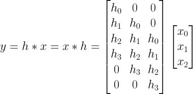
The matrix representing the incremental delays of used in the above equation is a special form of matrix called Toeplitz matrix. Toeplitz matrix have constant entries along their diagonals. Toeplitz matrices are used to model systems that posses shift invariant properties. The property of shift invariance is evident from the matrix structure itself. Since we are modelling a Linear Time Invariant system[1], Toeplitz matrices are our natural choice. On a side note, a special form of Toeplitz matrix called “circulant matrix” is used in applications involving circular convolution and Discrete Fourier Transform (DFT)[2].
Representing the operation used to construct the Toeplitz matrix out of the sequence  as
as  ,
,

Now, the convolution of and is simply a matrix multiplication of Toeplitz matrix  and the matrix representation of denoted as

One can quickly vectorize the convolution operation in matlab by using Toeplize matrices as shown below.
y=toeplitz([h0 h1 h2 h3 0 0],[h0 0 0])*x.';
Continue reading on “methods to compute linear convolution“…
For understanding the usage of toeplitz command in Matlab refer [3]
Rate this article: 
 (18 votes, average: 4.44 out of 5)
References:
[1] Reddi.S.S,”Eigen Vector properties of Toeplitz matrices and their application to spectral analysis of time series”, Signal Processing, Vol 7,North-Holland, 1984,pp 46-56.↗
[2] Robert M. Gray,”Toeplitz and circulant matrices – an overview”,Deptartment of Electrical Engineering,Stanford University,Stanford 94305,USA.↗
[3] Matlab documentation help on Toeplitz command.↗
Topics in this chapter
Books by the author
 Wireless Communication Systems in Matlab Second Edition(PDF)  (168 votes, average: 3.71 out of 5) (168 votes, average: 3.71 out of 5) |  Digital Modulations using Python (PDF ebook) (124 votes, average: 3.60 out of 5) |  Digital Modulations using Matlab (PDF ebook) (129 votes, average: 3.71 out of 5) |
| Hand-picked Best books on Communication Engineering Best books on Signal Processing |
||