Why BLUE :
We have discussed Minimum Variance Unbiased Estimator (MVUE) in one of the previous articles. Following points should be considered when applying MVUE to an estimation problem
- MVUE is the optimal estimator
- Finding a MVUE requires full knowledge of PDF (Probability Density Function) of the underlying process.
- Even if the PDF is known, finding an MVUE is not guaranteed.
- If PDF is unknown, it is impossible find an MVUE using techniques like Cramer Rao Lower Bound (CRLB)
- In practice, knowledge of PDF of the underlying process is actually unknown.
Considering all the points above, the best possible solution is to resort to finding a sub-optimal estimator. When we resort to find a sub-optimal estimator
- We may not be sure how much performance we have lost – Since we will not able to find the MVUE estimator for bench marking (due to non-availability of underlying PDF of the process).
- We can live with it, if the variance of the sub-optimal estimator is well with in specification limits
Common Approach for finding sub-optimal Estimator:
- Restrict the estimator to be linear in data
- Find the linear estimator that is unbiased and has minimum variance
- This leads to Best Linear Unbiased Estimator (BLUE)
- To find a BLUE estimator, full knowledge of PDF is not needed. Just the first two moments (mean and variance) of the PDF is sufficient for finding the BLUE
Definition of BLUE:
Consider a data set ![x[n]= \{ x[0],x[1], \cdots ,x[N-1] \}](https://s0.wp.com/latex.php?latex=x%5Bn%5D%3D+%5C%7B+x%5B0%5D%2Cx%5B1%5D%2C+%5Ccdots+%2Cx%5BN-1%5D+%5C%7D+&bg=ffffff&fg=000&s=0&c=20201002) whose parameterized PDF
whose parameterized PDF  depends on the unknown parameter
  . As the BLUE restricts the estimator to be linear in data, the estimate of the parameter can be written as linear combination of data samples with some weights
![\hat{\theta} = \displaystyle{\sum_{n=0}^{N} a_n x[n] = \textbf{a}^T \textbf{x}} \quad\quad \rightarrow (1)](https://s0.wp.com/latex.php?latex=%5Chat%7B%5Ctheta%7D+%3D+%5Cdisplaystyle%7B%5Csum_%7Bn%3D0%7D%5E%7BN%7D+a_n+x%5Bn%5D+%3D+%5Ctextbf%7Ba%7D%5ET+%5Ctextbf%7Bx%7D%7D+%C2%A0%5Cquad%5Cquad+%5Crightarrow+%281%29+&bg=ffffff&fg=000&s=2&c=20201002)
Here  is a vector of constants whose value we seek to find in order to meet the design specifications. Thus, the entire estimation problem boils down to finding the vector of constants – . The above equation may lead to multiple solutions for the vector . However, we need to choose those set of values of , that provides estimates that are unbiased and has minimum variance.
Thus seeking the set of values for  for finding a BLUE estimator that provides minimum variance, must satisfy the following two constraints
- The estimator must be linear in data
- Estimate must be unbiased
Constraint 1: Linearity Constraint:
Linearity constraint was already given above. Just repeated here for convenience.
![\hat{\theta} = \displaystyle{\sum_{n=0}^{N} a_n x[n] = \textbf{a}^T \textbf{x}} \quad\quad (1)](https://s0.wp.com/latex.php?latex=%5Chat%7B%5Ctheta%7D+%3D+%5Cdisplaystyle%7B%5Csum_%7Bn%3D0%7D%5E%7BN%7D+a_n+x%5Bn%5D+%3D+%5Ctextbf%7Ba%7D%5ET+%5Ctextbf%7Bx%7D%7D+%C2%A0%5Cquad%5Cquad%C2%A0%281%29+&bg=ffffff&fg=000&s=2&c=20201002)
Constraint 2: Constraint for unbiased estimates:
For the estimate to be considered unbiased, the expectation (mean) of the estimate must be equal to the true value of the estimate.
![E[\hat{\theta}] = \theta \quad\quad (2)](https://s0.wp.com/latex.php?latex=E%5B%5Chat%7B%5Ctheta%7D%5D+%3D+%5Ctheta+%5Cquad%5Cquad%C2%A0%282%29+&bg=ffffff&fg=000&s=2&c=20201002)
Thus,
![\displaystyle{\sum_{n=0}^{N} a_n E \left( x[n] \right) = \theta} \quad\quad (3)](https://s0.wp.com/latex.php?latex=%5Cdisplaystyle%7B%5Csum_%7Bn%3D0%7D%5E%7BN%7D+a_n+E+%5Cleft%28%C2%A0x%5Bn%5D+%5Cright%29%C2%A0%3D%C2%A0%5Ctheta%7D%C2%A0%5Cquad%5Cquad+%283%29+&bg=ffffff&fg=000&s=2&c=20201002)
Combining both the constraints (1) and (2) or (3),
![E[\hat{\theta}] =\displaystyle{\sum_{n=0}^{N} a_n E \left( x[n] \right) = \textbf{a}^T \textbf{x} = \theta} \quad\quad (4)](https://s0.wp.com/latex.php?latex=E%5B%5Chat%7B%5Ctheta%7D%5D+%3D%5Cdisplaystyle%7B%5Csum_%7Bn%3D0%7D%5E%7BN%7D+a_n+E+%5Cleft%28+x%5Bn%5D+%5Cright%29+%C2%A0%3D+%5Ctextbf%7Ba%7D%5ET+%5Ctextbf%7Bx%7D%C2%A0%C2%A0%3D%C2%A0%5Ctheta%7D%C2%A0%5Cquad%5Cquad+%284%29%C2%A0&bg=ffffff&fg=000&s=2&c=20201002)
Now, the million dollor question is : “When can we meet both the constraints ? “. We can meet both the constraints only when the observation is linear. That is ![x[n]](https://s0.wp.com/latex.php?latex=x%5Bn%5D&bg=ffffff&fg=000&s=0&c=20201002) is of the form
is of the form ![x[n]=s[n] \theta](https://s0.wp.com/latex.php?latex=x%5Bn%5D%3Ds%5Bn%5D+%5Ctheta+&bg=ffffff&fg=000&s=0&c=20201002) , where is the unknown parameter that we wish to estimate.
, where is the unknown parameter that we wish to estimate.
Consider a data model, as shown below, where the observed samples are in linear form with respect to the parameter to be estimated.
![x[n] = s[n] \theta + w[n] \quad\quad (5)](https://s0.wp.com/latex.php?latex=x%5Bn%5D+%3D+s%5Bn%5D+%5Ctheta+%2B+w%5Bn%5D+%C2%A0%5Cquad%5Cquad+%285%29+&bg=ffffff&fg=000&s=2&c=20201002)
Here , ![w[n]](https://s0.wp.com/latex.php?latex=w%5Bn%5D&bg=ffffff&fg=000&s=0&c=20201002) is zero mean process noise , whose PDF can take any form (Uniform, Gaussian, Colored etc., ). The mean of the above equation is given by
is zero mean process noise , whose PDF can take any form (Uniform, Gaussian, Colored etc., ). The mean of the above equation is given by
![E(x[n]) = E(s[n] \theta) = s[n] \theta \quad\quad(6)](https://s0.wp.com/latex.php?latex=E%28x%5Bn%5D%29+%3D+E%28s%5Bn%5D+%5Ctheta%29+%3D+s%5Bn%5D+%5Ctheta%C2%A0%C2%A0%5Cquad%5Cquad%286%29+&bg=ffffff&fg=000&s=2&c=20201002)
Substuiting (6) in (4) ,
![E[\hat{\theta}] = \displaystyle{\sum_{n=0}^{N} a_n E \left( x[n] \right) = \theta \sum_{n=0}^{N} a_n s[n] = \theta \textbf{a}^T \textbf{s} = \theta} \quad\quad (7)](https://s0.wp.com/latex.php?latex=E%5B%5Chat%7B%5Ctheta%7D%5D+%3D+%5Cdisplaystyle%7B%5Csum_%7Bn%3D0%7D%5E%7BN%7D+a_n+E+%5Cleft%28+x%5Bn%5D+%5Cright%29+%3D+%5Ctheta+%5Csum_%7Bn%3D0%7D%5E%7BN%7D+a_n+s%5Bn%5D+%3D+%5Ctheta+%5Ctextbf%7Ba%7D%5ET+%5Ctextbf%7Bs%7D+%3D+%5Ctheta%7D+%5Cquad%5Cquad+%287%29+&bg=ffffff&fg=000&s=2&c=20201002)
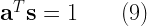
Looking at the last set of equality,
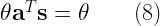
The above equality can be satisfied only if
Given this condition is met, the next step is to minimize the variance of the estimate. Minimizing the variance of the estimate,
![\begin{aligned} var(\hat{\theta})&=E\left [ \left (\sum_{n=0}^{N}a_n x[n] - E\left [\sum_{n=0}^{N}a_n x[n] \right ] \right )^2 \right ]\\ &=E\left [ \left ( \textbf{a}^T \textbf{x} - \textbf{a}^T E[\textbf{x}] \right )^2\right ]\\ &=E\left [ \left ( \textbf{a}^T \left [\textbf{x}- E(\textbf{x}) \right ] \right )^2\right ]\\ &=E\left [ \textbf{a}^T \left [\textbf{x}- E(\textbf{x}) \right ]\left [\textbf{x}- E(\textbf{x}) \right ]^T \textbf{a} \right ]\\ &=E\left [ \textbf{a}^T \textbf{C} \textbf{a} \right ]\\ &=\textbf{a}^T \textbf{C} \textbf{a} \end{aligned} \quad\quad (10)](https://s0.wp.com/latex.php?latex=%5Cbegin%7Baligned%7D+var%28%5Chat%7B%5Ctheta%7D%29%26%3DE%5Cleft+%5B+%5Cleft+%28%5Csum_%7Bn%3D0%7D%5E%7BN%7Da_n+x%5Bn%5D+-+E%5Cleft+%5B%5Csum_%7Bn%3D0%7D%5E%7BN%7Da_n+x%5Bn%5D+%5Cright+%5D+%5Cright+%29%5E2+%5Cright+%5D%5C%5C+%26%3DE%5Cleft+%5B+%5Cleft+%28+%5Ctextbf%7Ba%7D%5ET+%5Ctextbf%7Bx%7D+-+%5Ctextbf%7Ba%7D%5ET+E%5B%5Ctextbf%7Bx%7D%5D+%5Cright+%29%5E2%5Cright+%5D%5C%5C+%26%3DE%5Cleft+%5B+%5Cleft+%28+%5Ctextbf%7Ba%7D%5ET+%5Cleft+%5B%5Ctextbf%7Bx%7D-+E%28%5Ctextbf%7Bx%7D%29+%5Cright+%5D+%5Cright+%29%5E2%5Cright+%5D%5C%5C+%26%3DE%5Cleft+%5B+%5Ctextbf%7Ba%7D%5ET+%5Cleft+%5B%5Ctextbf%7Bx%7D-+E%28%5Ctextbf%7Bx%7D%29+%5Cright+%5D%5Cleft+%5B%5Ctextbf%7Bx%7D-+E%28%5Ctextbf%7Bx%7D%29+%5Cright+%5D%5ET+%5Ctextbf%7Ba%7D+%5Cright+%5D%5C%5C+%26%3DE%5Cleft+%5B+%5Ctextbf%7Ba%7D%5ET+%5Ctextbf%7BC%7D+%5Ctextbf%7Ba%7D+%5Cright+%5D%5C%5C+%26%3D%5Ctextbf%7Ba%7D%5ET+%5Ctextbf%7BC%7D+%5Ctextbf%7Ba%7D+%5Cend%7Baligned%7D+%5Cquad%5Cquad+%2810%29+&bg=ffffff&fg=000&s=2&c=20201002)
Finding BLUE:
As discussed above, in order to find a BLUE estimator for a given set of data, two constraints – linearity & unbiased estimates – must be satisfied and the variance of the estimate should be minimum. Thus the goal is to minimize the variance of  which is
  subject to the constraint
  . This is a typical Lagrangian Multiplier↗ problem, which can be considered as minimizing the following equation with respect to (Remember !!! this is what we would like to find ).

Minimizing  with respect to is equivalent to setting the first derivative of w.r.t to zero.

Substituting (12) in (9)

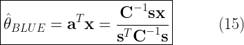
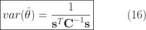
Finally, from (12) and (13), the co-effs of the BLUE estimator (vector of constants that weights the data samples) is given by

The BLUE estimate and the variance of the estimates are as follows
Rate this article: 
 (33 votes, average: 4.24 out of 5)
Similar topics
Books by the author
 Wireless Communication Systems in Matlab Second Edition(PDF)  (169 votes, average: 3.70 out of 5) (169 votes, average: 3.70 out of 5) |  Digital Modulations using Python (PDF ebook) (125 votes, average: 3.61 out of 5) |  Digital Modulations using Matlab (PDF ebook) (130 votes, average: 3.68 out of 5) |
| Hand-picked Best books on Communication Engineering Best books on Signal Processing |
||