A brief intro to modeling a frequency selective fading channel using tapped delay line (TDL) filters. Rayleigh & Rician frequency-selective fading channel models explained.
Tapped delay line filters
Tapped-delay line filters (FIR filters) are best to simulate multiple echoes originating from same source. Hence they can be used to model multipath scenarios. Tapped-Delay-Line (TDL) filters with  number taps can be used to simulate a multipath frequency selective fading channel. Frequency selective channels are characterized by time varying nature of the channel. For simulating a frequency selective channel, it is mandatory to have N > 1. In contrast, if N = 1, it simulates a zero-mean fading channel where all the multipath signals arrive at the receiver at the same time.
This article is part of the book Wireless Communication Systems in Matlab, ISBN: 978-1720114352 available in ebook (PDF) format (click here) and Paperback (hardcopy) format (click here).
Let  be the associated path attenuation corresponding to the received power
  and propagation delay
  of the
  th path. In continuous time, the complex path attenuation is given by
![\displaystyle{\tilde{a_n}(t) = a_n(t) exp\left[ -j 2 \pi f_c \tau_n(t) \right]}](https://s0.wp.com/latex.php?latex=%5Cdisplaystyle%7B%5Ctilde%7Ba_n%7D%28t%29+%3D+a_n%28t%29+exp%5Cleft%5B+-j+2+%5Cpi+f_c+%5Ctau_n%28t%29+%5Cright%5D%7D+&bg=ffffff&fg=000&s=2&c=20201002)
The complex channel response is given by
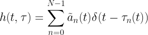
In the equation above, the attenuation and path delay vary with time. This simulates a time-variant complex channel.
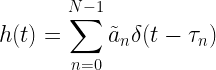
As a special case, in the absence any movements or other changes in the transmission channel, the channel can remain fairly time invariant (fixed channel with respect to instantaneous time  ) even though the multipath is present. Thus the time-invariant complex channel becomes
Usually, the pair  is described as a Power Delay Profile (PDP) plot. A sample power delay profile plot for a fixed, discrete, three ray model with its corresponding implementation using a tapped-delay line filter is shown in the following figure

 and
andpropagation delays
 are fixed)
Choose underlying distribution:
The next level of modeling involves, introduction of randomness in the above mentioned model there by rendering the channel response time variant. If the path attenuations are typically drawn from a complex Gaussian random variable, then at any given time , the absolute value of the impulse response  is
is
● Rayleigh distributed – if the mean of the distribution ![E [h(t; \tau)] = 0](https://s0.wp.com/latex.php?latex=E+%5Bh%28t%3B+%5Ctau%29%5D+%3D+0&bg=ffffff&fg=000&s=0&c=20201002)
● Rician distributed – if the mean of the distribution ![E [h(t; \tau)] \neq 0](https://s0.wp.com/latex.php?latex=E+%5Bh%28t%3B+%5Ctau%29%5D+%5Cneq+0&bg=ffffff&fg=000&s=0&c=20201002)
Respectively, these two scenarios model the presence or absence of a Line of Sight (LOS) path between the transmitter and the receiver. The first propagation delay  has no effect on the model behavior and hence it can be removed.
Similarly, the propagation delays can also be randomized, resulting in a more realistic but extremely complex model to implement. Furthermore, the power-delay-profile specifications with arbitrary time delays, warrant non-uniformly spaced tapped-delay-line filters, that are not suitable for practical simulation. For ease of implementation, the given PDP model with arbitrary time delays can be converted to tractable uniformly spaced statistical model by a combination of interpolation/approximation/uniform-sampling of the given power-delay-profile.
Real-life modelling:
Usually continuous domain equations for modeling multipath are specified in standards like COST-207 model in GSM specification. Such continuous time power-delay-profile models can be simulated using discrete-time Tapped Delay Line (TDL) filter with number of taps with variable tap gains. Given the order , the problem boils down to determining the discrete tap spacing  and the path gains , in such a way that the simulated channel closely follows the specified multipath PDP characteristics. A survey of method to find a solution for this problem can be found in [2].
Rate this article: 

 (10 votes, average: 3.80 out of 5)
References:
[1] Julius O. Smith III, Physical Audio Signal Processing, W3K Publishing, 2010, ISBN 978-0-9745607-2-4.↗
[2] M. Paetzold, A. Szczepanski, N. Youssef, Methods for Modeling of Specified and Measured Multipath Power-Delay Profiles, IEEE Trans. on Vehicular Techn., vol.51, no.5, pp.978-988, Sep.2002.↗
Topics in this chapter
| Small-scale Models for Multipath Effects ● Introduction ● Statistical characteristics of multipath channels □ Mutipath channel models □ Scattering function □ Power delay profile □ Doppler power spectrum □ Classification of small-scale fading ● Rayleigh and Rice processes □ Probability density function of amplitude □ Probability density function of frequency ● Modeling frequency flat channel ● Modeling frequency selective channel □ Method of equal distances (MED) to model specified power delay profiles □ Simulating a frequency selective channel using TDL model |
Books by the author
 Wireless Communication Systems in Matlab Second Edition(PDF) (169 votes, average: 3.70 out of 5) |  Digital Modulations using Python (PDF ebook) (125 votes, average: 3.61 out of 5) |  Digital Modulations using Matlab (PDF ebook) (130 votes, average: 3.68 out of 5) |
| Hand-picked Best books on Communication Engineering Best books on Signal Processing |
||
Hi!
I was looking for ways to model different channels in Octave/Matlab to simulate OFDM systems and, as I had read some interesting posts here, I bought the second edition of “Simulation of Digital Communication Systems Using Matlab”.
However, I miss examples of combining PDP with Rayleigh and Rician models, as well as frequency-selective channel models. Could you please provide examples?
By reading this post and the book, I think I could do something like the following code.
If I understood correctly, this code models a frequency-selective time-invariant Rayleigh channel with a know PDP.
Is it right?
—————————————————
%After the generation of the symbols in the time domain – vector “s”
%Channel model
pdp = [.6 .3 .1]; %channel with three taps
noise_power=.2;
h_i = randn(1,length(pdp));
h_q = randn(1,length(pdp));
h = sqrt ( pdp / 2 ) .* (h_i+j*h_q); %channel as TDL
s_channel = conv(h, s);
n_i = randn(1,length(s_channel));
n_q = randn(1,length(s_channel));
n = sqrt ( noise_power / 2 ) .* (n_i+j*n_q); %AWGN noise
s_channel_noise = s_channel + n;
—————————————————
Your code is more or less close. However, you have to make adjustments to normalize the output power of the TDL filter to unity, this is to make overall channel path gain to unity.
In the following code, the factor 1/sqrt(2) to normalize the Rayleigh fading variables and 1/sqrt(sum(pdp)) is to normalize the output power of the TDL filter to unity.
%Frequency Selective Rayleigh Block Fading TDL model (uniformly spaced taps)
%Assuming the given PDP values are already in linear scale
L=5000; %number of channel realizations, change this to 1 if only one realization is needed
N = length(PDP); %number of channel taps
a = sqrt(PDP); %path gains (tap coefficients a[n])
%Rayleigh a set of random variables R0,R1,R2,…R{N-1} with unit average power
%for each channel realization (block type fading)
R =1/sqrt(2)*(randn(L,N) + 1i*randn(L,N)); % normalized the Rayleigh fading variables
taps= repmat(a,L,1).*R; %combined tap weights = a[n]*R[n]
h= 1/sqrt(sum(PDP))*taps;%Normalized taps for output with unit average power
Now, you can use the rest of the code as
s_channel = conv(h,s)
… so on
Hi!
Thanks for yous prompt answer.
What do you mean by “number of channel realizations”?
If I keep your code, the channel h becomes a matrix of size LxN, which can not be convolved.
How should I filter the transmitted signal?
My objective is measuring the BER by generating several frames, and each frame is composed by several OFDM symbols, but the complete transmitted signal is just the concatenation of all those frames?
What is the best approach?
“channel realization” means capturing the random variations of the channel at a particular time instant. If there are 2 realizations, it means it captures how the channel behaves at two different time instances.
If I intend to transmit 2 OFDM frame, I could do it in two ways
1) Generate 1 OFDM frame at a time, set L=1 and generate random channel samples of length N , convolve it with the OFDM frame and receive it for processing at the receiver. Loop this two times and accumulate the BER statistics.
2) Generate 2 OFDM frames, set L=2 and generate random channel samples of length 2xN , convolve it with the OFDM frames and receive them for processing at the receiver. No loop needed in this case.
For OFDM type simulations and due to limited memory in computers, we can keep things simple and transmit only 1 OFDM frame at a time. In this case we are only interested in 1 channel realization. Due to the nature of the random variable, the samples of the channel realization would randomly change for one OFDM frame to next frame.
As commented in the code, the L can be set 1 . This is to avoid confusion in implementing the convolution and loop the transmission->channel realization->reception for every frame.
By the way, the ebook does have a chapter on OFDM, where I have used the approach (1) discussed above.
Thank you very much for the complete explanation!
I will use your first approach in my simulations.
What do you mean by “The first propagation delay τ0τ0 has no effect on the model behavior and hence it can be removed”?
The first delay block in the filter has no effect on the output. With or without this delay block, the output will remain same. It can be removed.
In the TDL representation of the three ray model, shouldn’t x(t) enter tau_0, tau_1, and tau_2 blocks?
The way it was represented, shouldn’t the block labels be tau_0, (tau_1 – tau_0), and (tau_2 – tau_1 – tau_0)?
Thanks!
The filter delays should be marked ∆τ. ∆ is missing in the diagram. Yes, it the difference between the current delay and the previous delay.
What is the physical significance of “channel tap” in a Raleigh fading channel ? Is it related to number of paths and how to determine the number of taps?
As the single tap flat fading channel is implemented as
Data_length=length(Data); %% Data is any signal
ray = sqrt(0.5*((randn(1,Data_length)).^2+(randn(1,PAR.Data_length)).^2));
Data_sent = Data.*ray;
Now, If I want to model a 6 tap frequency selective channel, how can I modify the above MATLAB code ?
For a flat fading channel tap is taken as 1. For frequency selective fading, the channel taps (N>1) can be obtained from the power delay profile. Power delay profile (PDP) plot contains the intensity of the received signal in a multipath environment plotted against the delta delay (difference in travel time between multipath arrivals).
The multi-tap channel need to implemented using an FIR filter, where the number of FIR taps depend on the maximum excess delay computed from the PDP. (see here: https://www.gaussianwaves.com/2014/07/power-delay-profile/ ). Once the number of taps are determined, there are methods to determine the tap coefficients and the time delays in the FIR filter. This is topic more complex to describe in the comment section. You could refer the following paper for more details.
M. Paetzold, A. Szczepanski, N. Youssef, Methods for Modeling of Specified and Measured Multipath Power-Delay Profiles,
IEEE Trans. on Vehicular Techn., vol.51, no.5, pp.978-988, Sep.2002
Thank you..
Can we consider number of paths=number of taps ?