Phase demodulation via Hilbert transform: Hands-on

Key focus: Demodulation of phase modulated signal by extracting instantaneous phase can be done using Hilbert transform. Hands-on demo in Python & Matlab.

Phase modulated signal:

The concept of instantaneous amplitude/phase/frequency are fundamental to information communication and appears in many signal processing application. We know that a monochromatic signal of form x(t) = a cos(ω t + ɸ) cannot carry any information. To carry information, the signal need to be modulated. Different types of modulations can be performed – amplitude modulation, phase modulation / frequency modulation.

In amplitude modulation, the information is encoded as variations in the amplitude of a carrier signal. Demodulation of an amplitude modulated signal, involves extraction of envelope of the modulated signal. This was discussed and demonstrated here.

[table “47” not found /]

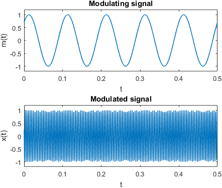
In phase modulation, the information is encoded as variations in the phase of the carrier signal. In its generic form, a phase modulated signal is expressed as an information-bearing sinusoidal signal modulating another sinusoidal carrier signal

\[x(t) = A cos \left[ 2 \pi f_c t + \beta + \alpha sin \left( 2 \pi f_m t + \theta \right) \right]   \quad \quad \quad (1)\]

where, m(t) = α sin (2 π f_m t + θ ) represents the information-bearing modulating signal, with the following parameters

α – amplitude of the modulating sinusoidal signal
f_m – frequency of the modulating sinusoidal signal
θ – phase offset of the modulating sinusoidal signal

The carrier signal has the following parameters

A – amplitude of the carrier
f_c – frequency of the carrier and f_c>>f_m
β – phase offset of the carrier

Demodulating a phase modulated signal:

The phase modulated signal shown in equation (1), can be simply expressed as

\[x(t) = A cos \left[ \phi(t) \right]    \quad\quad\quad (2) \]

Here,  ɸ(t) is the instantaneous phase  that varies according to the information signal m(t).

A phase modulated signal of form x(t) can be demodulated by forming an analytic signal by applying Hilbert transform and then extracting the instantaneous phase. This method is explained here.

We note that the instantaneous phase is ɸ(t) = 2 π f_c t + β + α sin (2 π f_m t + θ) is linear in time, that is proportional to 2 π f_c t . This linear offset needs to be subtracted from the instantaneous phase to obtained the information bearing modulated signal. If the carrier frequency is known at the receiver, this can be done easily. If not, the carrier frequency term 2 π f_c t needs to be estimated using a linear fit of the unwrapped instantaneous phase. The following Matlab and Python codes demonstrate all these methods.

Matlab code

%Demonstrate simple Phase Demodulation using Hilbert transform
clearvars; clc;
fc = 240; %carrier frequency
fm = 10; %frequency of modulating signal
alpha = 1; %amplitude of modulating signal
theta = pi/4; %phase offset of modulating signal
beta = pi/5; %constant carrier phase offset 
receiverKnowsCarrier= 'False'; %If receiver knows the carrier frequency & phase offset

fs = 8*fc; %sampling frequency
duration = 0.5; %duration of the signal
t = 0:1/fs:1-1/fs; %time base

%Phase Modulation
m_t = alpha*sin(2*pi*fm*t + theta); %modulating signal
x = cos(2*pi*fc*t + beta + m_t ); %modulated signal

figure(); subplot(2,1,1)
plot(t,m_t) %plot modulating signal
title('Modulating signal'); xlabel('t'); ylabel('m(t)')

subplot(2,1,2)
plot(t,x) %plot modulated signal
title('Modulated signal'); xlabel('t');ylabel('x(t)')

%Add AWGN noise to the transmitted signal
nMean = 0; %noise mean
nSigma = 0.1; %noise sigma
n = nMean + nSigma*randn(size(t)); %awgn noise
r = x + n;  %noisy received signal

%Demodulation of the noisy Phase Modulated signal
z= hilbert(r); %form the analytical signal from the received vector
inst_phase = unwrap(angle(z)); %instaneous phase

%If receiver don't know the carrier, estimate the subtraction term
if strcmpi(receiverKnowsCarrier,'True')
    offsetTerm = 2*pi*fc*t+beta; %if carrier frequency & phase offset is known
else
    p = polyfit(t,inst_phase,1); %linearly fit the instaneous phase
    estimated = polyval(p,t); %re-evaluate the offset term using the fitted values
    offsetTerm = estimated;
end
    
demodulated = inst_phase - offsetTerm;

figure()
plot(t,demodulated); %demodulated signal
title('Demodulated signal'); xlabel('n'); ylabel('\hat{m(t)}');

Python code

import numpy as np
from scipy.signal import hilbert
import matplotlib.pyplot as plt
PI = np.pi

fc = 240 #carrier frequency
fm = 10 #frequency of modulating signal
alpha = 1 #amplitude of modulating signal
theta = PI/4 #phase offset of modulating signal
beta = PI/5 #constant carrier phase offset 
receiverKnowsCarrier= False; #If receiver knows the carrier frequency & phase offset

fs = 8*fc #sampling frequency
duration = 0.5 #duration of the signal
t = np.arange(int(fs*duration)) / fs #time base

#Phase Modulation
m_t = alpha*np.sin(2*PI*fm*t + theta) #modulating signal
x = np.cos(2*PI*fc*t + beta + m_t ) #modulated signal

plt.figure()
plt.subplot(2,1,1)
plt.plot(t,m_t) #plot modulating signal
plt.title('Modulating signal')
plt.xlabel('t')
plt.ylabel('m(t)')
plt.subplot(2,1,2)
plt.plot(t,x) #plot modulated signal
plt.title('Modulated signal')
plt.xlabel('t')
plt.ylabel('x(t)')

#Add AWGN noise to the transmitted signal
nMean = 0 #noise mean
nSigma = 0.1 #noise sigma
n = np.random.normal(nMean, nSigma, len(t))
r = x + n  #noisy received signal

#Demodulation of the noisy Phase Modulated signal
z= hilbert(r) #form the analytical signal from the received vector
inst_phase = np.unwrap(np.angle(z))#instaneous phase

#If receiver don't know the carrier, estimate the subtraction term
if receiverKnowsCarrier:
    offsetTerm = 2*PI*fc*t+beta; #if carrier frequency & phase offset is known
else:
    p = np.poly1d(np.polyfit(t,inst_phase,1)) #linearly fit the instaneous phase
    estimated = p(t) #re-evaluate the offset term using the fitted values
    offsetTerm = estimated
                           
demodulated = inst_phase - offsetTerm 

plt.figure()
plt.plot(t,demodulated) #demodulated signal
plt.title('Demodulated signal')
plt.xlabel('n')
plt.ylabel('\hat{m(t)}')

Results

Rate this article: [ratings]

For further reading

[1] V. Cizek, “Discrete Hilbert transform”, IEEE Transactions on Audio and Electroacoustics, Volume: 18 , Issue: 4 , December 1970.↗

Topics in this chapter

[table “31” not found /]

Books by the author

[table “23” not found /]