From Maxwell’s equations to antenna array – part 1

Key focus: Briefly look at the building blocks of antenna array theory starting from the fundamental Maxwell’s equations in electromagnetism.

Maxwell’s equations

Maxwell’s equations are a collection of equations that describe the behavior of electromagnetic fields. The equations relate the electric fields () and magnetic fields () to their respective sources – charge density () and current density ( ).

Maxwell’s equations are available in two forms: differential form and integral form. The integral forms of Maxwell’s equations are helpful in their understanding the physical significance.

Maxwell’s equation (1):

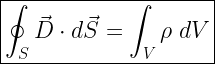
The flux of the displacement electric field through a closed surface equals the total electric charge enclosed in the corresponding volume space .

This is also called Gauss law for electricity.

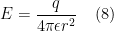
Consider a point charge +q in a three dimensional space. Assuming a symmetric field around the charge and at a distance r from the charge, the surface area of the sphere is .

Figure 1: Illustration of Coulomb’s law using Maxwell’s equation

Therefore, left side of the equation is simply equal to the surface area of the sphere multiplied by the magnitude of the electric displacement vector .

For the right hand side of the Maxwell’s equation (1), the integral of the charge density over a volume V is simply equal to the charge enclosed. Therefore,

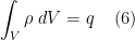
The electric displacement field is a measure of electric field in the material after taking into account the effect of the material on the electric field. The electric field and the displacement field are related by the permittivity of the material as

Combining equations (5), (6) and (7), yields the magnitude of an electric field as derived from Coulomb’s law

Maxwell’s equation (2)

The flux of the magnetic field through a closed surface is zero. That is, the net of magnetic field that “flows into” and “flows out of” a closed surface is zero.

This implies that there are no source or sink for the magnetic flux lines, in other words – they are closed field lines with no beginning or end. This is also called Gauss law for magnetic field.

Gauss law for magnetic field
Figure 2: Gauss law for magnetic field

Maxwell’s equation (3)

The work done on an electric charge as it travels around a closed loop conductor is the electromotive force (emf). Therefore, the left side of the gives the emf induced in a circuit.

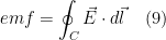
The right side of the equation is the rate of change of magnetic flux through the circuit.

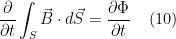
Hence, the Maxwell’s third equation is actually the Faraday’s (and Len’s) law of magnetic induction

The electromotive force (emf) induced in a circuit is directly proportional to the rate of change of magnetic flux through the circuit.

Figure 3: Faraday’s law for magnetic induction

Maxwell’s equation (4)

The circulating magnetic field is denoted by the circulation of magnetizing field around a closed curved path : . The electric current is denoted by the flux of current density () through any surface spanning that curved path. The quantity denotes the rate of change of displacement current through any surface spanning that curved path.

According to Maxwell’s extension to the Ampere’s law , magnetic fields can be generated in two ways: with electric current and with changing electric flux. The equation states that the electric current or change in electric flux through a surface produces a circulating magnetic field around any path that bounds that surface.

Summary of Maxwell’s equations

The electric field leaving a volume space is proportional to the electric charge contained in the volume.

The net of magnetic field that “flows into” and “flows out of” a closed surface is zero. There is no concept called magnetic charge/magnetic monopole.

A changing magnetic flux through a circuit induces electromotive force in the circuit

Magnetic fields are produced by electric current as well as by changing electric flux.

Rate this article: Note: There is a rating embedded within this post, please visit this post to rate it.

References

[1] The Feynman lectures on physics – online edition ↗

Books by the author


Wireless Communication Systems in Matlab
Second Edition(PDF)

Note: There is a rating embedded within this post, please visit this post to rate it.
Checkout Added to cart

Digital Modulations using Python
(PDF ebook)

Note: There is a rating embedded within this post, please visit this post to rate it.
Checkout Added to cart

Digital Modulations using Matlab
(PDF ebook)

Note: There is a rating embedded within this post, please visit this post to rate it.
Checkout Added to cart
Hand-picked Best books on Communication Engineering
Best books on Signal Processing

Normalized power gain of dipole antennas

Key focus: Briefly look at linear antennas and various dipole antennas and plot the normalized power gain pattern in polar plot and three dimensional plot.

Linear antennas

Linear antennas are electrically thin antennas whose conductor diameter is very small compared to the wavelength of the radiation λ.

Viewed in a spherical coordinate system (Figure 1), for linear antenna, the antenna is oriented along the z-axis such that the radiation vector has only components along directions of the radial distance Fr and the polar angle Fθ. The radiation vector is determined by the current density J which is characterized by the current distribution I(z) [1].

Figure 1: Electrical and magnetic fields from a current source
Figure 2: Linear antenna element

Hertzian dipole (infinitesimally small dipole)

Hertzian dipole is the simplest configuration of a linear antenna used for study purposes. It is an infinitesimally small (typically [2]) antenna element that has the following current density distribution

\[I(z) = I \; L\; \delta(z)\]

The radiation vector Fz (θ) is given by [1]

\[F_z(\theta) = \int_{-L/2}^{L/2} I(z^{'}) e^{jk_z z^{'}} dz{'} = \int_{-L/2}^{L/2} I L \delta(z{'}) e^{jkz{'}cos \theta} dz{'} = IL\]

The normalized power gain of the Hertzian dipole is [2]

\[g(\theta) = C_0 sin^{2} \theta \]

where, C0 is a constant chosen to make maximum of g(θ) equal to unity and θ is the polar angle in the spherical coordinate system.

Center-fed dipole (standing wave antenna)

For the center-fed small dipole antenna, the current distribution is assumed to be a standing wave. Defining k = 2π/λ as the wave number and h = L/2 as the half-length of the antenna, the current distribution and the normalized power gain g(θ) are given by

\[I(z) = I \; sin \left[ k \left(L/2 – |z| \right) \right]\]
\[g(\theta) =C_n \left|\frac{cos (k h \; cos \theta) – cos( k h) }{sin \theta} \right| ^2\]

where, Cn is a constant chosen to make maximum of g(θ) equal to unity and θ is the polar angle in the spherical coordinate system.

Figure 3: Center-fed small dipole

For half-wave dipole, set L = λ/2 or kl = π. Therefore, the current distribution for half-wave dipole shrinks to

\[I(z) = I \; cos(kz)\]

The normalized power gain is

\[g(\theta) = C_2 \frac{cos^2 (\frac{\pi}{2} cos \theta)}{sin^2 \theta} \approx C_2 sin^3 \theta\]

Plotting the normalized power gain

Let’s plot the normalized power gain pattern of Hertzian & Half-wave dipole antennas in polar plot and three dimensional plot.

Check out my Google colab for the python code to plot the normalized power gain in polar plot as well as three dimensional plot. The results are given below.

Figure 4: Hertzian dipole – power gain pattern (polar plot)
Figure 5: Hertzian dipole – power gain pattern (3D plot)
Figure 6: Half-wave dipole – power gain pattern (polar plot)
Figure 7: Half-wave dipole power gain 3d plot (cartesian coordinates)
Figure 8: Normalized power gain pattern for dipole of length
Figure 9: Normalized power gain pattern for dipole of length (3D projection)

Rate this article: Note: There is a rating embedded within this post, please visit this post to rate it.

References

[1] Orfanidis, S.J. (2013) Electromagnetic Waves and Antennas, Rutgers University. https://www.ece.rutgers.edu/~orfanidi/ewa/

[2] Constantine A. Balanis, Antenna Theory: Analysis and Design, ISBN: 978-1118642061, Wiley; 4th edition (February 1, 2016)