Retarded potentials

Key focus: Understand retarded potentials – the basic building block for understanding antenna array patterns. Retarded potentials are potentials at an observation point when the quantities at the source are non-static (varies in both space and time)

The static case : potentials

The fundamental premise of understanding antenna radiation is to understand how a radiation source influences the propagation of travelling electromagnetic waves. Propagation of travelling waves are best described by electric and magnetic potentials along the propagation path.

In the static case, the electric field E, charge density ρ, current density J and the electric potential Φ , magnetic field B and magnetic potential A are all constant in time. That is, they are functions of radial distance r in the spherical co-ordinate system, but not functions of time t . The solution for Maxwell’s equations (in the spherical co-ordinate system) take the following equivalent form in terms of electric and magnetic potentials:

\[\begin{aligned} \Phi(r) & = \frac{1}{4 \pi \epsilon} \int_V \frac{\rho(r')}{R} d^3 r' \quad \quad (1) \\ A(r) & = \frac{\mu}{4 \pi} \int_V \frac{J(r’)}{R} d^3 r’ \quad \quad (2) \end{aligned}\]
Potentials - solutions for Maxwell's equations for static case
Figure 1: Potentials – solutions for Maxwell’s equations for static case

The quantity R is the distance between the source and the point at which the corresponding fields are observed and d3 r’ is the volume element at the source point.

The non-static case : retarded potentials

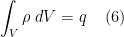
Since electromagnetic radiation are produced by time-varying electric charges, we are interested in describing the potentials at a given the observation point for this non-static situation. Obviously for the non-static case, the electric field E , charge density ρ , current density J and the electric potential Φ , magnetic field B and magnetic potential A are functions of both radial distance and time. The corresponding formulas for the potentials are

\[\begin{aligned} \Phi(r, t) & = \frac{1}{4 \pi \epsilon} \int_V \frac{\rho(r’, t – \frac{R}{c})}{R} d^3 r’ \quad \quad (3) \\ A(r, t) & = \frac{\mu}{4 \pi} \int_V \frac{J(r’, t – \frac{R}{c} )}{R} d^3 r’ \quad \quad (4) \end{aligned}\]

With c defined as the velocity of light, the factor t – R/c is the time delay between the emission of electromagnetic photon from the source and the time it gets observed by an observer. The electromagnetic field travels at certain velocity and hence the potentials at the observation point (due to the changing charge at source) are experienced after a certain time delay. Such potentials are called retarded potentials and the propagation delay t – R/c is called retarded time. Hence, we can say that the retarded potentials are related to electromagnetic fields of a current or charge distribution that vary in time.

Figure 2: Retarded potentials – solutions for Maxwell’s equations for non-static case

Sinusoidal time dependence of retarded potentials

In antenna theory, the antenna elements (source) are fed with sinusoidal waves. So, the next step is to express the retarded potentials at the observation point when all the quantities at source vary sinusoidally in time. Therefore, when the quantities are sinusoidal single-frequency waves, the shift property of Fourier transform can be applied.

\[\begin{aligned} \Phi(r, t) &= \Phi(r) e^{j \omega t} \\ \rho(r,t) &= \rho(r) e^{j \omega t} \\ A(r, t) &= A(r) e^{j \omega t} \\ J(r, t) &= J(r) e^{j \omega t} \end{aligned} \quad \quad (5)\]

Then, the retarded potential Φ(r,t) at the field observation point become,

\[\begin{aligned} \Phi(r, t) &= \frac{1}{4 \pi \epsilon} \int_V \frac{\rho(r', t – \frac{R}{c})}{R} d^3 r' \\ \Rightarrow \Phi(r) e^{j \omega t} & = \frac{1}{4 \pi \epsilon} \int_V \frac{\rho(r')e^{j \omega (t – \frac{R}{c})}}{R} d^3 r'\\ \Rightarrow \Phi(r) &= \frac{1}{4 \pi \epsilon} \int_V \frac{\rho(r')e^{-j \omega \frac{R}{c}}}{R} d^3 r'\\ \Rightarrow \Phi(r) &= \frac{1}{4 \pi \epsilon} \int_V \frac{\rho(r')e^{-j \frac{\omega}{c} R }}{R} d^3 r' \\ \Rightarrow \Phi(r) &= \frac{1}{4 \pi \epsilon} \int_V \frac{\rho(r')e^{-j k R }}{R} d^3 r' \end{aligned}\]

The retarded potential A(r,t) can be derived in a similar manner. Therefore, the retarded potentials (equations (3) and (4) ) for the single frequency sinusoidal wave is given by

\[\boxed{ \begin{aligned} \Phi(r) &= \frac{1}{4 \pi \epsilon} \int_V \frac{\rho(r')e^{-j k R }}{R} d^3 r' \\ A(r) &= \frac{\mu}{4 \pi} \int_V \frac{J(r')e^{-j k R }}{R} d^3 r' \end{aligned} }\]

In these equations, the quantity k = ω/c = 2 π/λ is called the free-space wavenumber.

Rate this article: Note: There is a rating embedded within this post, please visit this post to rate it.

Books by the author


Wireless Communication Systems in Matlab
Second Edition(PDF)

(173 votes, average: 3.66 out of 5)

Checkout Added to cart

Digital Modulations using Python
(PDF ebook)

(127 votes, average: 3.58 out of 5)

Checkout Added to cart

Digital Modulations using Matlab
(PDF ebook)

(134 votes, average: 3.63 out of 5)

Checkout Added to cart
Hand-picked Best books on Communication Engineering
Best books on Signal Processing

From Maxwell’s equations to antenna array – part 1

Key focus: Briefly look at the building blocks of antenna array theory starting from the fundamental Maxwell’s equations in electromagnetism.

Maxwell’s equations

Maxwell’s equations are a collection of equations that describe the behavior of electromagnetic fields. The equations relate the electric fields () and magnetic fields () to their respective sources – charge density () and current density ( ).

Maxwell’s equations are available in two forms: differential form and integral form. The integral forms of Maxwell’s equations are helpful in their understanding the physical significance.

Maxwell’s equation (1):

The flux of the displacement electric field through a closed surface equals the total electric charge enclosed in the corresponding volume space .

This is also called Gauss law for electricity.

Consider a point charge +q in a three dimensional space. Assuming a symmetric field around the charge and at a distance r from the charge, the surface area of the sphere is .

Figure 1: Illustration of Coulomb’s law using Maxwell’s equation

Therefore, left side of the equation is simply equal to the surface area of the sphere multiplied by the magnitude of the electric displacement vector .

For the right hand side of the Maxwell’s equation (1), the integral of the charge density over a volume V is simply equal to the charge enclosed. Therefore,

The electric displacement field is a measure of electric field in the material after taking into account the effect of the material on the electric field. The electric field and the displacement field are related by the permittivity of the material as

Combining equations (5), (6) and (7), yields the magnitude of an electric field as derived from Coulomb’s law

Maxwell’s equation (2)

The flux of the magnetic field through a closed surface is zero. That is, the net of magnetic field that “flows into” and “flows out of” a closed surface is zero.

This implies that there are no source or sink for the magnetic flux lines, in other words – they are closed field lines with no beginning or end. This is also called Gauss law for magnetic field.

Figure 2: Gauss law for magnetic field

Maxwell’s equation (3)

The work done on an electric charge as it travels around a closed loop conductor is the electromotive force (emf). Therefore, the left side of the gives the emf induced in a circuit.

The right side of the equation is the rate of change of magnetic flux through the circuit.

Hence, the Maxwell’s third equation is actually the Faraday’s (and Len’s) law of magnetic induction

The electromotive force (emf) induced in a circuit is directly proportional to the rate of change of magnetic flux through the circuit.

Figure 3: Faraday’s law for magnetic induction

Maxwell’s equation (4)

The circulating magnetic field is denoted by the circulation of magnetizing field around a closed curved path : . The electric current is denoted by the flux of current density () through any surface spanning that curved path. The quantity denotes the rate of change of displacement current through any surface spanning that curved path.

According to Maxwell’s extension to the Ampere’s law , magnetic fields can be generated in two ways: with electric current and with changing electric flux. The equation states that the electric current or change in electric flux through a surface produces a circulating magnetic field around any path that bounds that surface.

Summary of Maxwell’s equations

The electric field leaving a volume space is proportional to the electric charge contained in the volume.

The net of magnetic field that “flows into” and “flows out of” a closed surface is zero. There is no concept called magnetic charge/magnetic monopole.

A changing magnetic flux through a circuit induces electromotive force in the circuit

Magnetic fields are produced by electric current as well as by changing electric flux.

Rate this article: Note: There is a rating embedded within this post, please visit this post to rate it.

References

[1] The Feynman lectures on physics – online edition ↗

Books by the author


Wireless Communication Systems in Matlab
Second Edition(PDF)

Note: There is a rating embedded within this post, please visit this post to rate it.
Checkout Added to cart

Digital Modulations using Python
(PDF ebook)

Note: There is a rating embedded within this post, please visit this post to rate it.
Checkout Added to cart

Digital Modulations using Matlab
(PDF ebook)

Note: There is a rating embedded within this post, please visit this post to rate it.
Checkout Added to cart
Hand-picked Best books on Communication Engineering
Best books on Signal Processing