Tag: frequency sweep

Key focus: Know how to generate a Chirp signal, compute its Fourier Transform using FFT and power spectral density (PSD) in Matlab & Python.

This article is part of the following books ● Digital Modulations using Matlab : Build Simulation Models from Scratch, ISBN: 978-1521493885 ● Digital Modulations using Python ISBN: 978-1712321638 ● Wireless communication systems in Matlab ISBN: 979-8648350779 All books available in ebook (PDF) and Paperback formats

Introduction

All the signals discussed so far do not change in frequency over time. Obtaining a signal with time-varying frequency is of main focus here. A signal that varies in frequency over time is called “chirp”. The frequency of the chirp signal can vary from low to high frequency (up-chirp) or from high to low frequency (low-chirp).

Observation

Chirp signals/signatures are encountered in many applications ranging from radar, sonar, spread spectrum, optical communication, image processing, doppler effect, motion of a pendulum, as gravitation waves, manifestation as Frequency Modulation (FM), echo location ^[1] etc.

Mathematical Description:

A linear chirp signal sweeps the frequency from low to high frequency (or vice-versa) linearly. One approach to generate a chirp signal is to concatenate a series of segments of sine waves each with increasing(or decreasing) frequency in order. This method introduces discontinuities in the chirp signal due to the mismatch in the phases of each such segments. Modifying the equation of a sinusoid to generate a chirp signal is a better approach.

The equation for generating a sinusoidal (cosine here) signal with amplitude A, angular frequency and initial phase is

This can be written as a function of instantaneous phase

where is the instantaneous phase of the sinusoid and it is linear in time. The time derivative of instantaneous phase is equal to the angular frequency of the sinusoid – which in case is a constant in the above equation.

Instead of having the phase linear in time, let’s change the phase to quadratic form and thus non-linear.

for some constant .

Therefore, the equation for chirp signal takes the following form,

The first derivative of the phase, which is the instantaneous angular frequency becomes a function of time, which is given by

The time-varying frequency in Hertz is given by

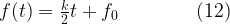
In the above equation, the frequency is no longer a constant, rather it is of time-varying nature with initial frequency given by . Thus, from the above equation, given a time duration T, the rate of change of frequency is given by

where, is the starting frequency of the sweep, is the frequency at the end of the duration T.

Substituting (7) & (8) in (6)

From (6) and (8)

where  is a constant which will act as the initial phase of the sweep.

Thus the modified equation for generating a chirp signal (from equations (5) and (10)) is given by

where the time-varying frequency function is given by

Generation of Chirp signal, computing its Fourier Transform using FFT and power spectral density (PSD) in Matlab is shown as example, for Python code, please refer the book Digital Modulations using Python.

Generating a chirp signal without using in-built “chirp” Function in Matlab:

Implement a function that describes the chirp using equation (11) and (12). The starting frequency of the sweep is and the frequency at time is . The initial phase forms the final part of the argument in the following function

function x=mychirp(t,f0,t1,f1,phase)
%Y = mychirp(t,f0,t1,f1) generates samples of a linear swept-frequency
%   signal at the time instances defined in timebase array t.  The instantaneous
%   frequency at time 0 is f0 Hertz.  The instantaneous frequency f1
%   is achieved at time t1.
%   The argument 'phase' is optional. It defines the initial phase of the
%   signal degined in radians. By default phase=0 radian
    
if nargin==4
    phase=0;
end
    t0=t(1);
    T=t1-t0;
    k=(f1-f0)/T;
    x=cos(2*pi*(k/2*t+f0).*t+phase);
end

The following wrapper script utilizes the above function and generates a chirp with starting frequency at the start of the time base and at which is the end of the time base. From the PSD plot, it can be ascertained that the signal energy is concentrated only upto 25 Hz

fs=500; %sampling frequency
t=0:1/fs:1; %time base - upto 1 second

f0=1;% starting frequency of the chirp
f1=fs/20; %frequency of the chirp at t1=1 second
x = mychirp(t,f0,1,f1); 
subplot(2,2,1)
plot(t,x,'k');
title(['Chirp Signal']);
xlabel('Time(s)');
ylabel('Amplitude');

FFT and power spectral density

As with other signals, describes in the previous posts, let’s plot the FFT of the generated chirp signal and its power spectral density (PSD).

L=length(x);
NFFT = 1024;
X = fftshift(fft(x,NFFT));
Pxx=X.*conj(X)/(NFFT*NFFT); %computing power with proper scaling
f = fs*(-NFFT/2:NFFT/2-1)/NFFT; %Frequency Vector

subplot(2,2,2)
plot(f,abs(X)/(L),'r');
title('Magnitude of FFT');
xlabel('Frequency (Hz)')
ylabel('Magnitude |X(f)|');
xlim([-50 50])


Pxx=X.*conj(X)/(NFFT*NFFT); %computing power with proper scaling
subplot(2,2,3)
plot(f,10*log10(Pxx),'r');
title('Double Sided - Power Spectral Density');
xlabel('Frequency (Hz)')
ylabel('Power Spectral Density- P_{xx} dB/Hz');
xlim([-100 100])

X = fft(x,NFFT);
X = X(1:NFFT/2+1);%Throw the samples after NFFT/2 for single sided plot
Pxx=X.*conj(X)/(NFFT*NFFT);
f = fs*(0:NFFT/2)/NFFT; %Frequency Vector
subplot(2,2,4)
plot(f,10*log10(Pxx),'r');
title('Single Sided - Power Spectral Density');
xlabel('Frequency (Hz)')
ylabel('Power Spectral Density- P_{xx} dB/Hz');

References:

[1] Patrick Flandrin,“Chirps everywhere”,CNRS — Ecole Normale Supérieure de Lyon

Topics in this chapter

Essentials of Signal Processing ● Generating standard test signals  □ Sinusoidal signals  □ Square wave  □ Rectangular pulse  □ Gaussian pulse  □ Chirp signal ● Interpreting FFT results - complex DFT, frequency bins and FFTShift  □ Real and complex DFT  □ Fast Fourier Transform (FFT)  □ Interpreting the FFT results  □ FFTShift  □ IFFTShift ● Obtaining magnitude and phase information from FFT  □ Discrete-time domain representation  □ Representing the signal in frequency domain using FFT  □ Reconstructing the time domain signal from the frequency domain samples ● Power spectral density ● Power and energy of a signal  □ Energy of a signal  □ Power of a signal  □ Classification of signals  □ Computation of power of a signal - simulation and verification ● Polynomials, convolution and Toeplitz matrices  □ Polynomial functions  □ Representing single variable polynomial functions  □ Multiplication of polynomials and linear convolution  □ Toeplitz matrix and convolution ● Methods to compute convolution  □ Method 1: Brute-force method  □ Method 2: Using Toeplitz matrix  □ Method 3: Using FFT to compute convolution  □ Miscellaneous methods ● Analytic signal and its applications  □ Analytic signal and Fourier transform  □ Extracting instantaneous amplitude, phase, frequency  □ Phase demodulation using Hilbert transform ● Choosing a filter : FIR or IIR : understanding the design perspective  □ Design specification  □ General considerations in design

Books by the author

Wireless Communication Systems in Matlab Second Edition(PDF) Note: There is a rating embedded within this post, please visit this post to rate it. $14.99 – Add to Cart Checkout Added to cart	Digital Modulations using Python (PDF ebook) Note: There is a rating embedded within this post, please visit this post to rate it. $14.99 – Add to Cart Checkout Added to cart	Digital Modulations using Matlab (PDF ebook) Note: There is a rating embedded within this post, please visit this post to rate it. $14.99 – Add to Cart Checkout Added to cart
Hand-picked Best books on Communication Engineering Best books on Signal Processing