Understanding Analytic Signal and Hilbert Transform

Key focus of this article: Understand the relationship between analytic signal, Hilbert transform and FFT. Hands-on demonstration using Python and Matlab.

Introduction

Fourier Transform of a real-valued signal is complex-symmetric. It implies that the content at negative frequencies are redundant with respect to the positive frequencies. In their works, Gabor [1] and Ville [2], aimed to create an analytic signal by removing redundant negative frequency content resulting from the Fourier transform. The analytic signal is complex-valued but its spectrum will be one-sided (only positive frequencies) that preserved the spectral content of the original real-valued signal. Using an analytic signal instead of the original real-valued signal, has proven to be useful in many signal processing applications. For example, in spectral analysis, use of analytic signal in-lieu of the original real-valued signal mitigates estimation biases and eliminates cross-term artifacts due to negative and positive frequency components [3].

This article is part of the following books ● Digital Modulations using Matlab : Build Simulation Models from Scratch, ISBN: 978-1521493885 ● Digital Modulations using Python ISBN: 978-1712321638 ● Wireless communication systems in Matlab ISBN: 979-8648350779 All books available in ebook (PDF) and Paperback formats

Continuous-time analytic signal

Let be a real-valued non-bandlimited finite energy signal, for which we wish to construct a corresponding analytic signal .  The Continuous Time Fourier Transform of is given by

Lets say the magnitude spectrum of is as shown in Figure 1(a). We note that the signal is a real-valued and its magnitude spectrum is symmetric and extends infinitely in the frequency domain.

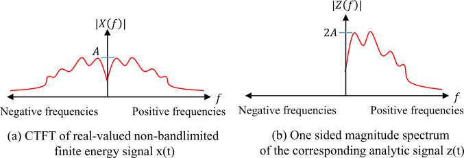
As mentioned in the introduction, an analytic signal can be formed by suppressing the negative frequency contents of the Fourier Transform of the real-valued signal. That is, in frequency domain, the spectral content of the analytic signal is given by

The corresponding spectrum of the resulting analytic signal is shown in Figure 1(b).

Since the spectrum of the analytic signal is one-sided, the analytic signal will be complex valued in the time domain, hence the analytic signal can be represented in terms of real and imaginary components as . Since the spectral content is preserved in an analytic signal, it turns out that the real part of the analytic signal in time domain is essentially the original real-valued signal itself . Then, what takes place of the imaginary part ? Who is the companion to x(t) that occupies the imaginary part in the resulting analytic signal ? Summarizing as equation,

It is interesting to note that Hilbert transform [4] can be used to find a companion function (imaginary part in the equation above) to a real-valued signal such that the real signal can be analytically extended from the real axis to the upper half of the complex plane . Denoting Hilbert transform as , the analytic signal is given by

From these discussion, we can see that an analytic signal for a real-valued signal , can be constructed using two approaches.

●  Frequency domain approach: The one-sided spectrum of is formed from the two-sided spectrum of the real-valued signal by applying equation (2)
● Time domain approach: Using Hilbert transform approach given in equation (4)

One of the important property of an analytic signal is that its real and imaginary components are orthogonal

Discrete-time analytic signal

Since we are in digital era, we are more interested in discrete-time signal processing. Consider a continuous real-valued signal gets sampled at interval seconds and results in real-valued discrete samples , i.e, . The spectrum of the continuous signal is shown in Figure 2(a). The spectrum of that results from the process of periodic sampling is given in Figure 2(b) (Refer here more details on the process of sampling).  The spectrum of discrete-time signal can be obtained by Discrete-Time Fourier Transform (DTFT).

At this point, we would like to construct a discrete-time analytic signal from the real-valued sampled signal . We wish the analytic signal is complex valued and should satisfy the following two desired properties

● The real part of the analytic signal should be same as the original real-valued signal.
● The real and imaginary part of the analytic signal should satisfy the following property of orthogonality

In Frequency domain approach for the continuous-time case, we saw that an analytic signal is constructed  by suppressing the negative frequency components from the spectrum of the real signal. We cannot do this for our periodically sampled signal . Periodic mirroring nature of the spectrum prevents one from suppressing the negative components. If we do so, it will vanish the entire spectrum. One solution to this problem is to set the negative half of each spectral period to zero. The resulting spectrum of the analytic signal is shown in Figure 2(c).

Given a record of samples of even length , the procedure to construct the analytic signal is as follows. This method satisfies both the desired properties listed above.

● Compute the -point DTFT of using FFT
● N-point periodic one-sided analytic signal is computed by the following transform

● Finally, the analytic signal (z[n]) is obtained by taking the inverse DTFT of

Matlab

The given procedure can be coded in Matlab using the FFT function. Given a record of real-valued samples , the corresponding analytic signal can be constructed as given next. Note that the Matlab has an inbuilt function to compute the analytic signal. The in-built function is called hilbert.

function z = analytic_signal(x)
%x is a real-valued record of length N, where N is even %returns the analytic signal z[n]
x = x(:); %serialize
N = length(x);
X = fft(x,N);
z = ifft([X(1); 2*X(2:N/2); X(N/2+1); zeros(N/2-1,1)],N);
end

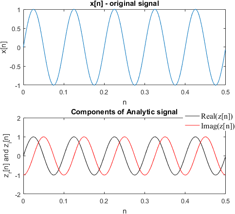
To test this function, we create a 5 seconds record of a real-valued sine signal. The analytic signal is constructed and the orthogonal components are plotted in Figure 3. From the plot, we can see that the real part of the analytic signal is exactly same as the original signal (which is the cosine signal) and the imaginary part of the analytic signal is phase shifted version of the original signal. We note that the imaginary part of the analytic signal is a cosine function with amplitude scaled by which is none other than the Hilbert transform of sine function.

t=0:0.001:0.5-0.001;
x = sin(2*pi*10*t); %real-valued f = 10 Hz
subplot(2,1,1); plot(t,x);%plot the original signal
title('x[n] - original signal'); xlabel('n'); ylabel('x[n]');

z = analytic_signal(x); %construct analytic signal
subplot(2,1,2); plot(t, real(z), 'k'); hold on;
plot(t, imag(z), 'r');
title('Components of Analytic signal'); 
xlabel('n'); ylabel('z_r[n] and z_i[n]');
legend('Real(z[n])','Imag(z[n])');

Python

Equivalent code in Python is given below (tested with Python 3.6.0)

import numpy as np
def main():
    t = np.arange(start=0,stop=0.5,step=0.001)
    x = np.sin(2*np.pi*10*t)
    
    import matplotlib.pyplot as plt
    plt.subplot(2,1,1)
    plt.plot(t,x)
    plt.title('x[n] - original signal')
    plt.xlabel('n')
    plt.ylabel('x[n]')
    
    z = analytic_signal(x)
    
    plt.subplot(2,1,2)
    plt.plot(t,z.real,'k',label='Real(z[n])')
    plt.plot(t,z.imag,'r',label='Imag(z[n])')
    plt.title('Components of Analytic signal')
    plt.xlabel('n')
    plt.ylabel('z_r[n] and z_i[n]')
    plt.legend()

def analytic_signal(x):
    from scipy.fftpack import fft,ifft
    N = len(x)
    X = fft(x,N)
    h = np.zeros(N)
    h[0] = 1
    h[1:N//2] = 2*np.ones(N//2-1)
    h[N//2] = 1
    Z = X*h
    z = ifft(Z,N)
    return z

if __name__ == '__main__':
    main()

Hilbert Transform using FFT

We should note that the hilbert function in Matlab returns the analytic signal $latex z[n]$ not the hilbert transform of the signal . To get the hilbert transform, we should simply get the imaginary part of the analytic signal. Since we have written our own function to compute the analytic signal, getting the hilbert transform of a real-valued signal goes like this.

x_hilbert = imag(analytic_signal(x))

In the coming posts, we will some of the applications of constructing an analytic signal. For example: Find the instantaneous amplitude and phase of a signal, envelope detector for an amplitude modulated signal, detecting phase changes in a sine wave.

Rate this article: (32 votes, average: 3.38 out of 5)

References:

[1] D. Gabor, “Theory of communications”, Journal of the Inst. Electr. Eng., vol. 93, pt. 111, pp. 42-57, 1946. See definition of complex signal on p. 432.↗
[2] J. A. Ville, “Theorie et application de la notion du signal analytique”, Cables el Transmission, vol. 2, pp. 61-74, 1948.↗
[3] S. M. Kay, “Maximum entropy spectral estimation using the analytical signal”, IEEE transactions on Acoustics, Speech, and Signal Processing, vol. 26, pp. 467-469, October 1978.↗
[4] Frank R. Kschischang, “The Hilbert Transform”, University of Toronto, October 22, 2006.↗
[5] S. L. Marple, “Computing the discrete-time ‘analytic’ signal via FFT,” Conference Record of the Thirty-First Asilomar Conference on Signals, Systems and Computers , Pacific Grove, CA, USA, 1997, pp. 1322-1325 vol.2.↗

Topics in this chapter

Essentials of Signal Processing ● Generating standard test signals  □ Sinusoidal signals  □ Square wave  □ Rectangular pulse  □ Gaussian pulse  □ Chirp signal ● Interpreting FFT results - complex DFT, frequency bins and FFTShift  □ Real and complex DFT  □ Fast Fourier Transform (FFT)  □ Interpreting the FFT results  □ FFTShift  □ IFFTShift ● Obtaining magnitude and phase information from FFT  □ Discrete-time domain representation  □ Representing the signal in frequency domain using FFT  □ Reconstructing the time domain signal from the frequency domain samples ● Power spectral density ● Power and energy of a signal  □ Energy of a signal  □ Power of a signal  □ Classification of signals  □ Computation of power of a signal - simulation and verification ● Polynomials, convolution and Toeplitz matrices  □ Polynomial functions  □ Representing single variable polynomial functions  □ Multiplication of polynomials and linear convolution  □ Toeplitz matrix and convolution ● Methods to compute convolution  □ Method 1: Brute-force method  □ Method 2: Using Toeplitz matrix  □ Method 3: Using FFT to compute convolution  □ Miscellaneous methods ● Analytic signal and its applications  □ Analytic signal and Fourier transform  □ Extracting instantaneous amplitude, phase, frequency  □ Phase demodulation using Hilbert transform ● Choosing a filter : FIR or IIR : understanding the design perspective  □ Design specification  □ General considerations in design

Books by the author

Wireless Communication Systems in Matlab Second Edition(PDF) (180 votes, average: 3.62 out of 5) $14.99 – Add to Cart Checkout Added to cart	Digital Modulations using Python (PDF ebook) (134 votes, average: 3.56 out of 5) $14.99 – Add to Cart Checkout Added to cart	Digital Modulations using Matlab (PDF ebook) (136 votes, average: 3.63 out of 5) $14.99 – Add to Cart Checkout Added to cart
Hand-picked Best books on Communication Engineering Best books on Signal Processing