
Energy & Spectra path: 1. Power & energy (you are here) → 2. Parseval’s theorem → 3. RMS value · Tool: Parseval demo
In one sentence: the energy of a signal is the total area under $|x(t)|^2$, and its power is the average of $|x(t)|^2$ over time. A signal with finite energy is an energy signal; a signal with finite, non-zero average power is a power signal.
The two formulas, side by side:
$$E_x = \int_{-\infty}^{\infty} |x(t)|^2, dt, \qquad P_x = \lim_{T to \infty} \frac{1}{2T} \int_{-T}^{T} |x(t)|^2, dt.$$
That’s really all there is to it. The rest of this article is about using them correctly: which one applies to which signal, worked examples you can check by hand, the difference between instantaneous and average power, and the one mistake almost everyone makes when computing energy from samples in Matlab or Python.
Why square the signal?
We want a single number that says how “big” a signal is. The plain area under $x(t)$ doesn’t work, because positive and negative parts cancel: a sine wave would have zero area. Taking the absolute value fixes that but is awkward to work with mathematically.
Squaring is the natural choice. It never cancels, it’s easy to differentiate, and it matches physics: if $x(t)$ is a voltage across a 1 Ω resistor, then $|x(t)|^2$ is exactly the power dissipated at time $t$. That’s why signal processing borrows the words energy and power.
Energy of a signal
For a continuous-time signal (real or complex):
$$E_x = \int_{-\infty}^{\infty} |x(t)|^2, dt.$$
For a discrete-time sequence:
$$E_x = \sum_{n=-\infty}^{\infty} |x[n]|^2.$$
If $x$ is real, $|x|^2$ is just $x^2$. For complex signals, $|x|^2 = x \cdot x^* = (\text{Re}, x)^2 + (\text{Im}, x)^2$.
A few examples you can work out with a pencil:
Rectangular pulse of height $A$ and width $\tau$:
$$E_x = \int_0^{\tau} A^2, dt = A^2 \tau.$$
Decaying exponential $x(t) = e^{-at}u(t)$ with $a > 0$:
$$E_x = \int_0^{\infty} e^{-2at}\, dt = \frac{1}{2a}.$$
Geometric sequence $x[n] = r^n u[n]$ with $|r| < 1$:
$$E_x = \sum_{n=0}^{\infty} r^{2n} = \frac{1}{1 – r^2}.$$
In every case the integral or sum converges, so these are energy signals.
From signal energy to joules
The formulas above give energy in “signal units”. To get physical energy, you need to know what $x(t)$ represents and what it drives. For a voltage $v(t)$ across a resistance $R$, and for a current $i(t)$ through it:
$$E = \frac{1}{R} \int_{-\infty}^{\infty} |v(t)|^2\, dt\, \qquad E = R \int_{-\infty}^{\infty} |i(t)|^2, dt.$$
With $R = 1 \Omega$ the signal energy and the physical energy are the same number.
Power of a signal
Some signals never die out. A sinusoid that runs forever has infinite energy, so energy is useless for describing it. Instead we ask: how much energy per second, on average? Take a window, measure the energy inside it, divide by the window length, and let the window grow:
$$P_x = \lim_{T \to\infty} \frac{1}{2T} \int_{-T}^{T} |x(t)|^2, dt.$$
The discrete-time version counts samples instead of seconds. A window from $-N$ to $N$ holds $2N + 1$ samples, which is where that slightly odd denominator comes from:
$$P_x = \lim_{N \to\infty} \frac{1}{2N + 1} \sum_{n=-N}^{N} |x[n]|^2.$$
You’ll also see the window written as $n = 0, \dots, N-1$ with a $1/N$ in front. It’s the same average with different indexing.
For a periodic signal you don’t need the limit at all. Every period looks the same, so averaging over one period $T_0$ gives the answer:
$$P_x = \frac{1}{T_0} \int_{0}^{T_0} |x(t)|^2\, dt.$$
Examples:
Sinusoid $x(t) = Acos(\omega_0 t + \phi)$. Using $cos^2\theta = \tfrac{1}{2}(1 + cos 2\theta)$, the $cos 2\theta$ part averages to zero:
$$P_x = \frac{A^2}{2}.$$
Complex exponential $x(t) = A e^{j\omega_0 t}$. Here $|x(t)|^2 = |A|^2$ at every instant, so
$$P_x = |A|^2.$$
Unit step $u(t)$. It’s 1 for half of any symmetric window and 0 for the other half:
$$P_x = \lim_{T to \infty} \frac{1}{2T} \int_{0}^{T} 1\, dt = \frac{1}{2}.$$
Sum of sinusoids at different frequencies, plus a DC offset $c$. The cross terms average out, so the powers simply add:
$$x(t) = c + \sum_k A_k cos(\omega_k t + \phi_k) \quad\Rightarrow\quad P_x = c^2 + \sum_k \frac{A_k^2}{2}.$$
Random noise with mean $\mu$ and variance $\sigma^2$:
$$P_x = \mu^2 + \sigma^2.$$
For zero-mean noise, power is just the variance. That’s the fact behind every noise-variance calculation in a BER simulation.
Energy signal vs power signal
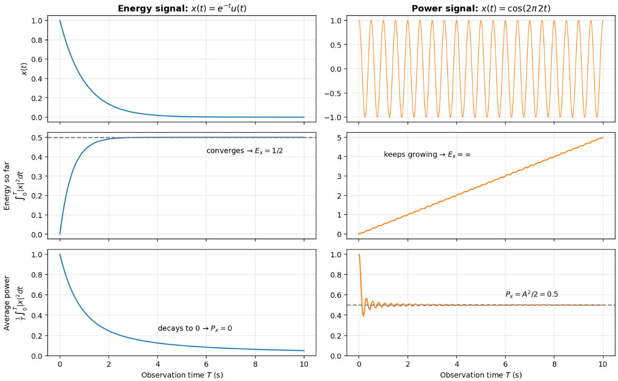
Figure 1 shows the difference better than any definition. On the left is a decaying pulse, on the right a sinusoid. The middle row is the energy collected up to time $T$, and the bottom row is that energy divided by $T$.

That gives the classification:
- Energy signal: $0 < E_x < \infty$. Its average power is then zero, because a finite amount of energy spread over infinite time averages out to nothing.
- Power signal: $0 < P_x < \infty$. Its energy is then infinite, because a non-zero rate sustained forever adds up to infinity.
- Neither: some signals have both $E_x$ and $P_x$ infinite. The ramp $x[n] = n$ is an example: it grows so fast that even its average blows up.
- Never both: a signal can’t have finite non-zero energy and finite non-zero power at the same time.
| Signal | Energy $E_x$ | Power $P_x$ | Type |
|---|---|---|---|
| Rectangular pulse, height $A$, width $\tau$ | $A^2\tau$ | $0$ | Energy |
| $e^{-at}u(t)$, $a > 0$ | $1/(2a)$ | $0$ | Energy |
| $Acos(\omega_0 t + \phi)$ | $\infty$ | $A^2/2$ | Power |
| $Ae^{j\omega_0 t}$ | $\infty$ | $\vert A \vert^2$ | Power |
| DC level $c$ | $\infty$ | $c^2$ | Power |
| Unit step $u(t)$ | $\infty$ | $1/2$ | Power |
| Zero-mean noise, variance $\sigma^2$ | $\infty$ | $\sigma^2$ | Power |
| Ramp $x[n] = n$ | $\infty$ | $\infty$ | Neither |
Instantaneous power, average power and RMS
There are really three related quantities, and mixing them up causes a lot of confusion:
- Instantaneous power $p(t) = |x(t)|^2$ is the power at one moment.
- Average power $P_x$ is the time average of $p(t)$.
- RMS value is the square root of the average power, $x_{\text{rms}} = \sqrt{P_x}$.

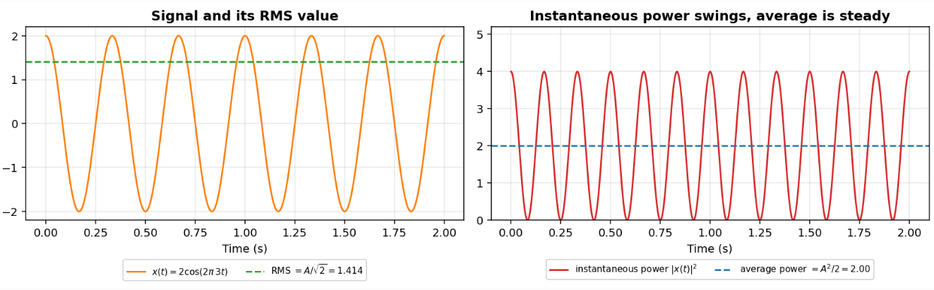
The RMS value is the constant level that would deliver the same average power. That’s why mains voltage is quoted as an RMS value: a 230 V RMS supply heats a resistor exactly as much as 230 V DC would.
Power is usually quoted in decibels. Relative to 1 watt (dBW) or 1 milliwatt (dBm):
$$P_{\text{dBW}} = 10\log_{10}\frac{P}{1 \text{W}}, \qquad P_{\text{dBm}} = 10\log_{10}\frac{P}{1 \text{mW}} = P_{\text{dBW}} + 30.$$
So 2 W is about 3.01 dBW, or 33.01 dBm.
Computing energy and power from samples
In a simulation you never have $x(t)$, only samples $x[n] = x(nT_s)$ taken every $T_s = 1/f_s$ seconds. Here’s the catch. To approximate the continuous-time energy, the sum needs a factor of $T_s$:
$$E_x \approx T_s \sum_{n} |x[n]|^2.$$
Leave out $T_s$ and your “energy” depends on how fast you sampled, which makes no physical sense.

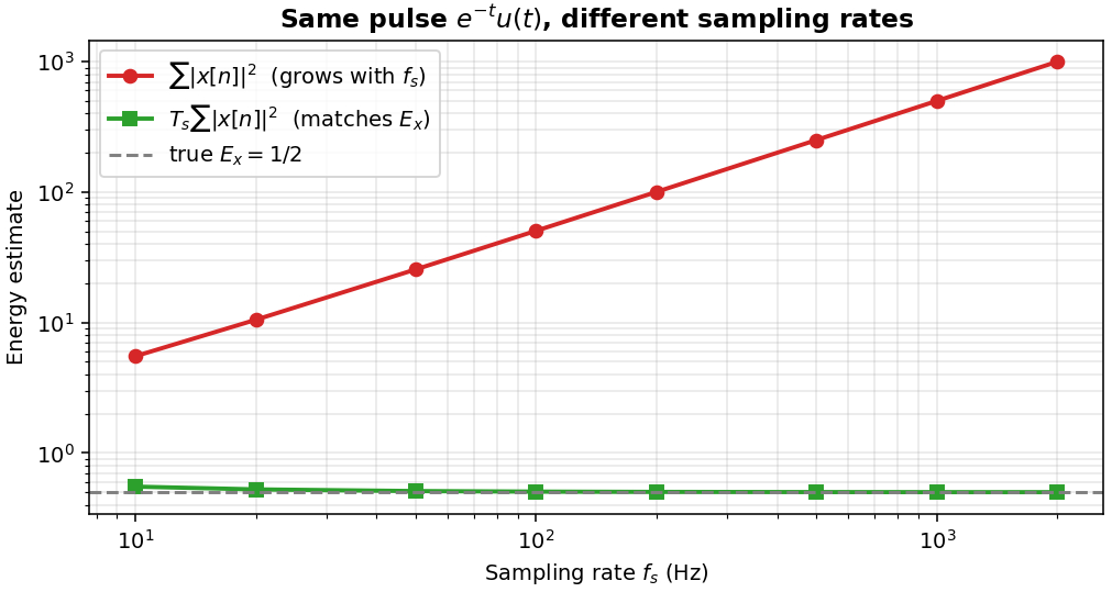
Average power doesn’t have this problem. The $T_s$ appears in both the energy and the duration ($N T_s$), so it cancels:
$$P_x \approx \frac{1}{N} \sum_{n=0}^{N-1} |x[n]|^2.$$
In code, that’s just the mean of the squared magnitude. One practical tip: for a periodic signal, use a whole number of periods, otherwise the leftover partial cycle biases the estimate slightly.
Python code
import numpy as np

def energy(x, fs):
    """Continuous-time energy estimate from samples taken at fs Hz."""
    return np.sum(np.abs(x)**2) / fs

def power(x):
    """Average power estimate from samples (independent of fs)."""
    return np.mean(np.abs(x)**2)

fs = 1000
t = np.arange(0, 20, 1/fs)

pulse = np.exp(-t)                    # energy signal, theory E = 1/2
print(f"Energy of exp(-t)u(t): {energy(pulse, fs):.4f}")

A = 2
sine = A * np.cos(2*np.pi*50*t)       # power signal, theory P = A^2/2 = 2
P = power(sine)
print(f"Power of 2cos(2*pi*50t): {P:.4f}")
print(f"RMS: {np.sqrt(P):.4f}, in dBm: {10*np.log10(P/1e-3):.2f} dBm")

rng = np.random.default_rng(1)
noise = np.sqrt(0.25) * rng.standard_normal(1_000_000)
print(f"Noise power: {power(noise):.4f} (variance 0.25)")Output:
Energy of exp(-t)u(t): 0.5005
Power of 2cos(2*pi*50t): 2.0000
RMS: 1.4142, in dBm: 33.01 dBm
Noise power: 0.2492 (variance 0.25)
The energy comes out as 0.5005 instead of 0.5 because a sum of samples only approximates the integral. Raise fs and it gets closer. The noise power wobbles around 0.25 from run to run, because it’s an estimate from random samples.
Matlab code
fs = 1000;  Ts = 1/fs;
t  = 0:Ts:20-Ts;

x  = exp(-t);                       % energy signal
Ex = Ts * sum(abs(x).^2);           % 0.5005 (theory 0.5)

A  = 2;
y  = A*cos(2*pi*50*t);              % power signal
Py = mean(abs(y).^2);               % 2.0000 (theory A^2/2)
yrms = sqrt(mean(y.^2));            % 1.4142
Py_dBm = 10*log10(Py/1e-3);         % 33.01 dBm

w  = sqrt(0.25)*randn(1, 1e6);      % zero-mean noise
Pw = mean(w.^2); % about 0.25 (the variance)For a step-by-step Matlab walkthrough, including checking power in the frequency domain, see Compute signal power in Matlab.
Questions readers often ask
An AM wave doesn’t last forever. Why do we calculate its power and not its energy? Because we model it as if it did. The equation $m(t)cos(2\pi f_c t)$ has no time limit in it, so mathematically it’s a power signal. In practice a transmission lasts far longer than any window you analyse, so average power is the useful number. If you deliberately limit it to $0 \le t \le t_0$, it becomes an energy signal.
Lightning is a short pulse with finite energy. Isn’t its power huge, not zero? Its instantaneous power is enormous. Its average power over all time is zero, because the finite energy is spread over an infinite interval. The classification in this article is about long-term average power, not peak power.
Why is the energy of a power signal infinite? A power signal keeps delivering energy at a non-zero average rate forever. Any non-zero rate multiplied by infinite time is infinite.
Why does the discrete power formula divide by $2N + 1$? The sum runs from $n = -N$ to $n = N$. That’s $N$ negative indices, $N$ positive ones and $n = 0$: $2N + 1$ samples in total.
My signal is from an accelerometer, not a voltage. What do I use for the load? Nothing. Without a load, the formulas give signal energy in the signal’s own units squared times seconds, here $(\text{m/s}^2)^2 \cdot \text{s}$. That’s perfectly fine for comparing signals or normalizing a simulation. Converting to joules needs a physical model of what the acceleration is driving.
How does Parseval’s theorem fit in? It says you get the same energy whether you integrate $|x(t)|^2$ in time or $|X(f)|^2$ in frequency. It’s a handy cross-check on FFT scaling. See Parseval’s theorem or try the Parseval demo.
Keep learning
- Parseval’s theorem — derivation: energy in time equals energy in frequency
- Significance of the RMS value
- Compute signal power in Matlab
- Simulation and analysis of white noise in Matlab
- Interpreting FFT results: magnitude and phase
- Eb/N0, Es/N0 and SNR converter: where signal and noise power meet in a link budget
Want the complete lab notebooks? The GaussianWaves ebooks bundle the Matlab and Python simulation code that goes beyond a single blog post.
References
- A. V. Oppenheim, A. S. Willsky and S. H. Nawab, Signals and Systems, 2nd ed., Prentice Hall, 1997, Section 1.1.2.
- S. Lall, “Norm and vector spaces,” Information Systems Laboratory, Stanford University.
So the finite energy signal’s power is Zero. I also refered http://cnx.org/content/m10055/latest/
Could you please explain why we calculate power relations in Amplitude Modulation ? AM wave is finite wave right? then its power should be zero. I know I am missing something, please correct me.
Energy signal is limited in time – bounding signal in time – example: rectangular pulse of finite duration.
On the otherhand, power signals are NOT limited in time – example sinusoid.
On the similar lines, an Amplitude modulated wave is a type of sinusoidal wave. When we write AM wave equation we simply write m(t)cos(2*pi*fc*t)
There is no time limit implied in this equation. Thus it is a qualifier for power signal and NOT an energy signal.
Suppose, if I define the same equation with a bound on time, m(t)cos(2*pi*fc*t) ; where t is between 0 and t0 – this makes the signal finite and therefore, this is NOT a power signal.
Energy signal has finite energy and zero power.Then the voltage generated by lightning is of short duration having finite energy but it has also large power.Is it right??please correct me if i m wrong
After the first formula is introduced, it states, that:
“If the signal x(t) is real, the modulus operator in the above equation does not matter.”
However, there is no modulus operator in the equation at all!
And second, how do I find the “load of a signal” so that I can convert to the real physical correspondent Energy?
For example, I’m currently working with accelerometer signals, so I measure in [g], or in [ms^-2]. Can someone tell me what the factor Z is in these cases?
Overall, thanks for the tutorial, it was very comprehensive!
Here, the modulus operator represents -‘absolute value’. It is indicated by |.| sign
If ‘x’ is complex, defined as xReal+j xImag, then |x| = sqrt(xReal^2 + xImag^2).
I am not sure about the accelerometer signal. But, in electrical engineering terms, usually the load is defined as the impedance that is driven by a source.
Thanks for the explanation, gives a general clue! I’ve got a question: is the even part of Ex (the energy function of a given x(t) signal) equal to Ex itself? The Ex even is 1/2 (int from -inf to inf |x(t)|^2 dt+ int from -inf to inf |x(-t)^2| dt) I believe that the integral from -inf to inf of |x(t)|^2 dt is equal to the integral from -inf to inf of |x(-t)|^2 dt for any given x(t). Thus making the Ex even = Ex, and Ex odd=0. Thanks!
Why do we take 1/2N+1 in discrete time power signal?
Summation takes samples from -N to +N indices, which is 2N+1 samples in total.
WHY IS THE ENERGY OF POWER SIGNAL INFINITE?
By definition, energy is the area under the squared signal. For power signal, example: periodic signals, the signal does not decay fast enough, hence the total area under the squared power signal will be infinite.