
FFT Lab path:
Complex DFT, bins & fftshift →
Magnitude & phase →
Spectral leakage →
ENBW
Plot: Matlab /
Python
· Tool: FFT bin & resolution calculator
In one sentence: after an FFT you hold complex bin values $latex X[k]=X_{\mathrm{re}}+jX_{\mathrm{im}}$; the magnitude $latex |X[k]|$ is the amplitude spectrum, and a trustworthy phase spectrum needs $latex \mathrm{atan2}$ plus a magnitude threshold so floating-point junk does not look like real angles.
This walk-through continues from complex DFT, frequency bins, and fftshift. We take a cosine with a known phase, compute an $latex N$-point FFT, plot magnitude and phase, then reconstruct the time signal.
Example signal
Use $latex A=0.5$, $latex f_c=10\,\mathrm{Hz}$, $latex \phi=30^{\circ}=\pi/6$:
\[x(t) = 0.5\,\cos(2\pi\cdot 10\,t + \pi/6)\]Sample at $latex f_s=32\,f_c=320\,\mathrm{Hz}$ (oversampling factor 32) for a 2 s record (640 samples). Nyquist sampling is covered here.
A = 0.5;              % amplitude
fc = 10;              % Hz
phase = 30;           % degrees
fs = 32*fc;           % 320 Hz
t = 0:1/fs:2-1/fs;    % 2 s
phi = phase*pi/180;
x = A*cos(2*pi*fc*t + phi);
plot(t, x);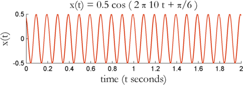
FFT: complex spectrum
Compute an $latex N$-point complex DFT. Choose $latex N$ large enough to cover the cycles you care about — here $latex N=256$ is enough for a pure tone. Matlab/NumPy’s fft omits the textbook $latex 1/N$ on the forward transform, so we scale by $latex 1/N$ to match the analysis definition. fftshift only reorders bins for a centered double-sided axis; it is optional for the math.
N = 256;
X = (1/N) * fftshift(fft(x, N));  % N-point complex DFT, centered
Magnitude (amplitude) spectrum
\[|X[k]| = \sqrt{X_{\mathrm{re}}^2 + X_{\mathrm{im}}^2}\]df = fs/N; % bin resolution (Hz)
sampleIndex = -N/2:N/2-1;
f = sampleIndex * df;
stem(f, abs(X));
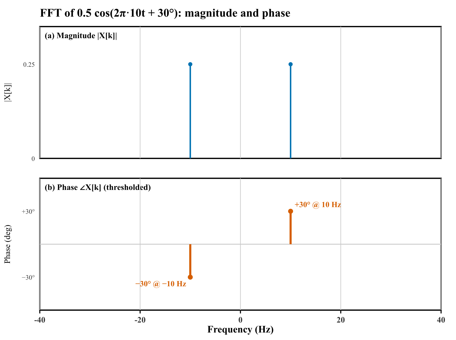
xlabel('f (Hz)'); ylabel('|X(k)|');For a real cosine of amplitude $latex A$, each of the two bins at $latex \pm f_c$ has height $latex A/2$ (here 0.25) after the $latex 1/N$ scaling — see Figure 3(a).

Phase spectrum — why it looks noisy
\[\angle X[k] = \mathrm{atan2}(X_{\mathrm{im}}, X_{\mathrm{re}})\]Use atan2 (four quadrants), not bare atan (only $latex [-\pi/2,\pi/2]$). Even then, bins that should be zero are tiny floats ($latex \sim 10^{-16}$). Their $latex \mathrm{atan2}$ ratio is random garbage — that is the “noisy phase” plot.
phase = atan2(imag(X), real(X)) * 180/pi;
plot(f, phase);  % looks like noise
Fix: zero out bins whose magnitude is below a fraction of the peak, then recompute phase.
X2 = X;
threshold = max(abs(X)) / 10000;
X2(abs(X) < threshold) = 0;
phase = atan2(imag(X2), real(X2)) * 180/pi;
plot(f, phase);
You should recover $latex +30^{\circ}$ at $latex +10\,\mathrm{Hz}$ and $latex -30^{\circ}$ at $latex -10\,\mathrm{Hz}$ (conjugate symmetry for real $latex x[n]$). Figure 3 combines magnitude and the cleaned phase.

Reconstruct the time signal
x_recon = N * ifft(ifftshift(X), N);
t = (0:length(x_recon)-1) / fs;
plot(t, x_recon);
Python twin
import numpy as np
import matplotlib.pyplot as plt

A, fc, phase_deg, fs, N = 0.5, 10.0, 30.0, 320.0, 256
t = np.arange(0, 2, 1 / fs)
x = A * np.cos(2 * np.pi * fc * t + np.deg2rad(phase_deg))

X = np.fft.fftshift(np.fft.fft(x[:N], N)) / N
f = np.fft.fftshift(np.fft.fftfreq(N, d=1 / fs))
mag = np.abs(X)
phase = np.angle(X, deg=True)
phase[mag < mag.max() / 10000] = 0.0

fig, ax = plt.subplots(2, 1, sharex=True, figsize=(8, 5))
ax[0].stem(f, mag, basefmt=" ")
ax[0].set_ylabel("|X[k]|")
ax[1].stem(f, phase, basefmt=" ")
ax[1].set_ylabel("Phase (deg)")
ax[1].set_xlabel("f (Hz)")
plt.show()

print("phase @ +10 Hz ≈", phase[np.argmin(np.abs(f - 10))], "deg")
Check bin spacing on the FFT resolution calculator. When windows enter the picture, correct the noise floor with ENBW.
FAQ
How do I convert an FFT bin index into hertz? For an $latex N$-point DFT at sampling rate $latex f_s$, bin $latex k$ corresponds to $latex f_k=k\,f_s/N$ (with bins $latex k>N/2$ representing negative frequencies when you use a two-sided layout). Always build the frequency axis from $latex f_s$ and $latex N$ rather than guessing from plot ticks.
Should I plot magnitude in linear units or dB? Linear magnitude is fine for spotting a single strong tone; dB (typically $latex 20\log_{10}|X|$) is better when you care about weak sidelobes, noise floor, or harmonic structure spanning many decades. Phase is meaningful only where the magnitude is well above the noise.
Why does my phase look random between peaks? In bins dominated by noise, the complex FFT value is essentially a random phasor, so the unwrapped phase wanders. Mask or ignore phase where $|X|$ is near the floor, and unwrap only across bins that belong to a real signal component.
how can I realize this in java?
I do not have the code in Java
While reconstructing the signal, what happens to the phase information. Since that is not being passed to the ifft(), how is the phase information restored in the time domain?
Hi Mathuranathan, thank you for this article, it’s very helpful. I’d like to extract the phase information from an OFDM signal. How can I do this? Thanks in advance
In OFDM, the phase estimation should be done after the FFT block in the receiver. Several algorithms/technique available for phase estimation in an OFDM system.
Consider a coherent detection system.
1. For each transmitted OFDM symbol, the FFT output contains say N modulated values (say QAM modulation is used)
2. These values may contain random phase shifts and amplitude variations caused by local oscillator drift, jitter, channel response and other factors.
3. We usually use a channel estimator (can be a pilot/preamble based one) to estimate the reference phases and amplitudes.
4. Once the reference phases and amplitudes are learnt, we can apply them to correct phase/amplitude errors in the actual data transmission.
You can take a look at this patent. I hope it offers more clue on how to use it for your system.
https://www.google.com/patents/US7423960
Thank you for your answer. In my system, an OFDM signal is used for extracting the distance between a TX and RX. The signal is composed solely by zadoff-chu pilots. I have extracted a coarse distance measure from the correlation function between the received signal and a refrence signal. Now I’d like to perform a fine estimation exploiting the signal phase estimated in frequency domain but I’m not able to do this.
This tutorial was amazing for me. Thank you for typing up the extremely clear presentation. I’m trying to understand the phase I’m getting – my data is an almost pure cosine from an RK4 algorithm but the phase has a discontinuity right at the frequency of the solution! https://uploads.disquscdn.com/images/f2af1d75093aad75bb03d8708d5ff80f9210bf52c02359728f17652e3d7e9745.jpg
is it really a pure cosine function ? is it possible to share the input data ?
Thanks !!!. Is it really a pure cosine function ? is it possible to share the input data ?
Thank you for the response. I found the answer – my solution had constant amplitude and frequency but was varying in phase over time, so the FFT accurately described my data.
—
Thanks for the explanation. If I increase N to 1024 or change fs to
20*fc, the magnitude and phase plots changes. Why does this happen? https://uploads.disquscdn.com/images/3b5435a0043d44b9c7682baf64b19d0f1f048f2271b682835bec2d02daa3b3e6.jpg
It is due to the spectral leakage. If the input signal is not periodic with respect to the length of FFT, it creates artifacts in the input signal that creates all these types of issues.
Examples here: https://www.gaussianwaves.com/2011/01/fft-and-spectral-leakage-2/
Hello Mathuranathan
Thank you very much for this article, I’ve a naive question, why when I try with a sine wave
x=A*sin(2*pi*fc*t+phi);
I get phase spectrum peak at 60 degree (pi/3) instead of 30 degree.
I’m not sure why this is happening do you have any clue?
Thank you
FFT does not know if the input signal is cosine or sine. We just compute the angle as the tan^-1(imaginary part/real part). The angle is always measured between the vector and the real axis.
https://uploads.disquscdn.com/images/d927e05add9359cb8c4691ef5df55c12cbfcbd486e98eb609a6dcd71dd909ee4.png
To give you clue, investigate the FFT output of a pure cosine wave and pure sine wave. Check the real part and imaginary part in each output, you will begin to understand
look at the following Matlab function, it can calculate phase spectrum as well as amplitude spectrum with a perfect accuracy:
https://www.mathworks.com/matlabcentral/fileexchange/63847-amplitude-and-phase-spectrum-of-a-signal–fourier-transform-
Great work !! it will definitely help everyone.
Thanks for this! I was wondering my my phase plot was not working. It turns out it was because of the atan function
Hi Mathuranathan, thank you for this article.
I have a doubt regarding calculation of DFT in matlab using DFT formulae and using inbulit MATLAB function FFT.
The
phase of DFT computed using DFT formula and FFT (inbuilt MATLAB
function) is different at N/2. Why is it so? Attaching sample code
clc;
close all;
clear all;
x = [2 3 -1 4];
N = length(x);
X = zeros(4,1)
%DFT formulae
for k = 0:N-1
for n = 0:N-1
X(k+1) = X(k+1) + x(n+1)*exp(-j*pi/2*n*k)
end
end
t = 0:N-1
subplot(311)
stem(t,x);
xlabel(‘Time (s)’);
ylabel(‘Amplitude’);
title(‘Time domain – Input sequence’)
%Magniltude Plot of DFT
magnitude=abs(X)
subplot(312);
stem(0:N-1,magnitude);
xlabel(‘Frequency’);
ylabel(‘|X(k)|’);
title(‘Magnitude Response’);
%Phase Plot of DFT
phase=atan2(imag(X),real(X))*180/pi
subplot(313)
stem(0:N-1,phase)
xlabel(‘Frequency’);
ylabel(‘Phase’);
title(‘Frequency domain – Phase response’)
%fft
figure;
X_k=fft(x,N)
t=0:N-1;
subplot(311)
stem(t,x);
xlabel(‘Time (s)’);
ylabel(‘Amplitude’);
title(‘Input sequence’)
%Magniltude Plot of DFT
magnitude=abs(X_k)
subplot(312);
stem(0:N-1,magnitude);
xlabel(‘Frequency’);
ylabel(‘|X(k)|’);
title(‘Magnitude Response’);
%Phase Plot of DFT
phase=atan2(imag(X_k),real(X_k))*180/pi
subplot(313);
stem(0:N-1,phase);
xlabel(‘Frequency’);
ylabel(‘Phase’);
title(‘Phase Response’);
Need a clarification. The plot below Section 3A has Y-axis label of X|f| whereas I think it has to be X|k|? Can you clarify?
Nice article. Thank you.
Is it possible to reconstruct the time domain signal while shiftted the phase from fft outputs?
Yes, it has to be X|k|.
Anyone knows how to change Matlab code into python? For the part where you apply the threshold thingy. I have tried doing it before but it doesn’t work
I loved this explanation. Really simple overview of FFT results. Plus, learned about phase, and all the tricks to view it properly. Beautifully done.
This example worked well until I changed the signal frequency and found the computed phase only to be correct when the sampling frequency is exactly a power of 2 higher than the signal frequency(x4,8,16,32,64 etc) otherwise it not correct. Is there some other correction that needs to be performed to the result in these cases?
This is due to spectral leakage phenomenon. You may read about it here
https://www.gaussianwaves.com/2011/01/fft-and-spectral-leakage-2/
Due to spectral leakage, you will see non-zero values for frequency components that are near the frequency of the signal. This will also reflect in the phase spectrum.
Set Fs=100 and N=length(x) (length(x)= 640 and it is not a power of 2). Now you will observe perfect frequency spectrum. However, if you change N=power of 2, spectrum will be affected by spectral leakage.
While doing the phase calculation from the above equation why i am getting more values than the input? I need that in same length.
The length of the phase vector (derived from FFT output) depends on the FFT length (N). In the example above the FFT length is set to 256. So it gives 256 phase values corresponding to 256 frequency bins.
The phase noise was driving me nuts! Already suspected something fishy with rounding errors but to no avail. The atan2 function did the trick for me! Thanks a lot!
Glad it worked for you!! Thank you !!!
Hi Mathuranathan,
Thanks for such an amazing article. It is very helpful in interpreting the data and understanding the Fourier Transform. Would you please help me interpreting the same for a 2D Fourier transform? Or can you please share any articles related to the 2D FFT or fft2(). It would be of great help.
Thanks again for such a vivid explanation of fft function.
The fundamentals are same for 2D Fourier transform. Its just that one more dimension is added to the processing. I suggest looking at this article
https://people.ciirc.cvut.cz/~hlavac/TeachPresEn/11ImageProc/12FourierTxEn.pdf
Why the amplitude in frequency domain is half of that in time domain?