Mathematical details of convolution, its relationship to polynomial multiplication and the application of Toeplitz matrices in computing linear convolution are discussed in the previous article. A short survey of different techniques to compute discrete linear convolution (with Matlab code) is given here.
Definition
Given an LTI (Linear Time Invariant) system with impulse response \(h[n]\) and an input sequence \(x[n]\), the output of the system \(y[n]\) is obtained by convolving the input sequence and impulse response.
where, the sequence \(x[n]\) is of length \(N\) and \(h[n]\) is of length \(M\).
This article is part of the following books |
Method 1 – Brute-Force Method:
The above equation can simply be implemented using nested for-loops, which consume the most computational time of all the methods given here. Typically, the computational complexity is \(O(n^2)\) time.
Python
def conv_brute_force(x,h):
	"""
	Brute force method to compute convolution
	Parameters:
	x, h : numpy vectors
	Returns:
		y : convolution of x and h
	"""
	N=len(x)
	M=len(h)
	y = np.zeros(N+M-1) #array filled with zeros

	for i in np.arange(0,N):
		for j in np.arange(0,M):
			y[i+j] = y[i+j] + x[i] * h[j]
return y
Matlab
for i = 0:n+m,
   yi = 0;
for i = 0 :n,
   for k = 0 to m,
      y[i+k] = y[i+k] + x[i] · h[k];
Method 2 – Using Toeplitz Matrix:
When the sequences \(h[n]\) and \(x[n]\) are represented as matrices, the linear convolution operation can be equivalently represented as
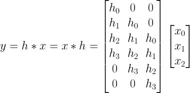
Assume that the sequence \(h[n]\) is of length 4 given by \(h[n]=[h_0,h_1,h_2,h_3]\) and the sequence \(x[n]\) is of length 3 given by \(x[n]=[x_0,x_1,x_2]\). The convolution \(h[n] \ast x[n]\) is given by
Equivalent representation of the above convolution can be written as
The matrix representing the incremental delays of \(h[n]\) used in the above equation is a special form of matrix called Toeplitz matrix. Toeplitz matrix have constant entries along their diagonals. Toeplitz matrices are used to model systems that posses shift invariant properties. The property of shift invariance is evident from the matrix structure itself. Since we are modelling a Linear Time Invariant system[1], Toeplitz matrices are our natural choice. On a side note, a special form of Toeplitz matrix called “circulant matrix” is used in applications involving circular convolution and Discrete Fourier Transform (DFT)[2].
For python code: refer the book – Digital modulations using Python
Matlab has inbuilt function to compute Toeplitz matrix from given vector. Toeplitz matrix of sequence \(h\) is given as
In Matlab, it is constructed by calling Toeplitz function[3] with two arguments. The first argument is the first column of the above matrix -\( [h_0,h_1,h_2,h_3,0,0]\) and the second argument is the first row of the above matrix – \([h_0,0,0]\).
y=toeplitz([h0 h1 h2 h3 0 0],[h0 0 0])*x.';
In the generalized case, where \(x\) and \(h\) are of any arbitrary lengths (say \(N\) and \(M\)), the code can be modified as follows [here it is assumed that \( length (x) \geq length(h)\) ]
k=toeplitz([h zeros(1,length(x)-1)],[h(1) zeros(1,length(x)-1])*x.'
Method 3: Using FFT:
Computation of convolution using FFT (Fast Fourier Transform) has the advantage of reduced computational complexity when the length of inputs are large. To compute convolution, take FFT of the two sequences \(x\) and \(h\) with FFT length set to convolution output length \(length (x)+length(h)-1\), multiply the results and convert back to time-domain using IFFT (Inverse Fast Fourier Transform). Note that FFT is a direct implementation of circular convolution in time domain. Here we are attempting to compute linear convolution using circular convolution (or FFT) with zero-padding either one of the input sequence. This causes inefficiency when compared to circular convolution. Nevertheless, this method still provides \(O\left(\frac{N}{log_2N}\right)\) savings over brute-force method.
Usually, the following algorithm is suffice which ignores additional zeros in the output terms.
Python
from scipy.fftpack import fft,ifft
y=ifft(fft(x,L)*(fft(h,L))) #Convolution using FFT and IFFT
Matlab
y=ifft(fft(x,L).*(fft(h,L)))
Other Methods:
If the input sequence is of infinite length or very very large as in many real time applications, block processing methods like Overlap-Add and Overlap-Save methods can be used to compute convolution in a faster and efficient way.
Standard Algorithms for Fast Convolution:
Standard algorithms for computing convolution that greatly reduce the computational complexity are
1) Cook-Toom Algorithm
2) Modified Cook-Toom Algorithm
3) Winograd Algorithm
4) Modified Winograd Algorithm
5) Iterated Convolution
Refer [4] -Fast Algorithms for Signal Processing by Richard E. Blahut for more details on the above algorithms (see reference section below).
Matlab Code
Implementing method 2 (convolution using Toeplitz matrix transformation) and method 3 (convolution using FFT) and comparing against Matlab’s standard conv function:
%Create random vectors for test
x=rand(1,7)+1i*rand(1,7);
h=rand(1,3)+1i*rand(1,3);
L=length(x)+length(h)-1;

%Convolution Using Toeplitz matrix
y1=toeplitz([h zeros(1,length(x)-1)],[h(1) zeros(1,length(x)-1)])*x.'
%Convolution FFT
y2=ifft(fft(x,L).*(fft(h,L))).'
%Matlab's standard function
y3=conv(h,x).'
Simulation output:
Comparing method 2 and method 3 against Matlab’s standard convolution function returns identical results
References:
[1] Reddi.S.S,”Eigen Vector properties of Toeplitz matrices and their application to spectral analysis of time series, Signal Processing, Vol 7, North-Holland, 1984, pp 46-56.↗
[2] Robert M. Gray,”Toeplitz and circulant matrices – an overview”,Deptartment of Electrical Engineering,Stanford University,Stanford 94305,USA.↗
[3] Matlab documentation help on Toeplitz command.↗
[4] Richard E. Blahut,”Fast Algorithms for Signal Processing”,ISBN-13: 978-0521190497,Cambridge University Press,August 16, 2010.↗
Topics in this chapter
Books by the author
 Wireless Communication Systems in Matlab Second Edition(PDF) Note: There is a rating embedded within this post, please visit this post to rate it. |  Digital Modulations using Python (PDF ebook) Note: There is a rating embedded within this post, please visit this post to rate it. |  Digital Modulations using Matlab (PDF ebook) Note: There is a rating embedded within this post, please visit this post to rate it. |
| Hand-picked Best books on Communication Engineering Best books on Signal Processing |
||


![a=[a_0,a_1,a_2,...,a_{n-1}]](https://s0.wp.com/latex.php?latex=a%3D%5Ba_0%2Ca_1%2Ca_2%2C...%2Ca_%7Bn-1%7D%5D&bg=ffffff&fg=000&s=0&c=20201002)

![a=[a_0,a_1,a_2,...,a_n]](https://s0.wp.com/latex.php?latex=a%3D%5Ba_0%2Ca_1%2Ca_2%2C...%2Ca_n%5D&bg=ffffff&fg=000&s=0&c=20201002)

![b=[b_0,b_1,b_2,...,b_n]](https://s0.wp.com/latex.php?latex=b%3D%5Bb_0%2Cb_1%2Cb_2%2C...%2Cb_n%5D&bg=ffffff&fg=000&s=0&c=20201002)


![p(x) . q(x)=(p\ast q)(x)=a.b=[c_0,c_1,c_2,\cdots,c_{n+m}] \; , \;where](https://s0.wp.com/latex.php?latex=p%28x%29+.+q%28x%29%3D%28p%5Cast+q%29%28x%29%3Da.b%3D%5Bc_0%2Cc_1%2Cc_2%2C%5Ccdots%2Cc_%7Bn%2Bm%7D%5D+%5C%3B+%2C+%5C%3Bwhere+&bg=ffffff&fg=000&s=2&c=20201002)


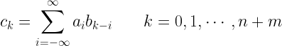

![c[k]=\displaystyle{\sum_{i=-\infty}^{\infty}a[i]b[k-i]} \quad\quad k=0,1,\cdots,n+m](https://s0.wp.com/latex.php?latex=c%5Bk%5D%3D%5Cdisplaystyle%7B%5Csum_%7Bi%3D-%5Cinfty%7D%5E%7B%5Cinfty%7Da%5Bi%5Db%5Bk-i%5D%7D+%5Cquad%5Cquad+k%3D0%2C1%2C%5Ccdots%2Cn%2Bm+&bg=ffffff&fg=000&s=2&c=20201002)


![h[n]](https://s0.wp.com/latex.php?latex=h%5Bn%5D&bg=ffffff&fg=000&s=0&c=20201002)
![x[n]](https://s0.wp.com/latex.php?latex=x%5Bn%5D&bg=ffffff&fg=000&s=0&c=20201002)

![y[n]](https://s0.wp.com/latex.php?latex=y%5Bn%5D&bg=ffffff&fg=000&s=0&c=20201002)

![y[k]=h[n]*x[n] = \displaystyle{\sum_{i=-\infty}^{\infty}x[i]h[k-i]}](https://s0.wp.com/latex.php?latex=y%5Bk%5D%3Dh%5Bn%5D%2Ax%5Bn%5D+%3D+%5Cdisplaystyle%7B%5Csum_%7Bi%3D-%5Cinfty%7D%5E%7B%5Cinfty%7Dx%5Bi%5Dh%5Bk-i%5D%7D+&bg=ffffff&fg=000&s=2&c=20201002)

![h[n]=[h_0,h_1,h_2,h_3]](https://s0.wp.com/latex.php?latex=h%5Bn%5D%3D%5Bh_0%2Ch_1%2Ch_2%2Ch_3%5D&bg=ffffff&fg=000&s=0&c=20201002)

![x[n]=[x_0,x_1,x_2]](https://s0.wp.com/latex.php?latex=x%5Bn%5D%3D%5Bx_0%2Cx_1%2Cx_2%5D&bg=ffffff&fg=000&s=0&c=20201002)

![h[n] \ast x[n]](https://s0.wp.com/latex.php?latex=h%5Bn%5D+%5Cast+x%5Bn%5D&bg=ffffff&fg=000&s=0&c=20201002)

![y[k]=h[n]*x[n] = \displaystyle{\sum_{i=-\infty}^{\infty}x[i]h[k-i]} \quad k=0,1,\cdots,5](https://s0.wp.com/latex.php?latex=y%5Bk%5D%3Dh%5Bn%5D%2Ax%5Bn%5D+%3D+%5Cdisplaystyle%7B%5Csum_%7Bi%3D-%5Cinfty%7D%5E%7B%5Cinfty%7Dx%5Bi%5Dh%5Bk-i%5D%7D+%5Cquad+k%3D0%2C1%2C%5Ccdots%2C5+&bg=ffffff&fg=000&s=2&c=20201002)


![\begin{bmatrix} y[0]\\y[1]\\y[2]\\y[3]\\y[4]\\y[5] \end{bmatrix}=\begin{bmatrix}h[0] &0 & 0 \\ h[1] & h[0] & 0 \\ h[2] & h[1] & h[0] \\ h[3] & h[2] & h[1] \\ 0 & h[3] & h[2] \\ 0 & 0 & h[3] \end{bmatrix} \begin{bmatrix}x[0]\\x[1]\\x[2] \end{bmatrix}](https://s0.wp.com/latex.php?latex=%5Cbegin%7Bbmatrix%7D+y%5B0%5D%5C%5Cy%5B1%5D%5C%5Cy%5B2%5D%5C%5Cy%5B3%5D%5C%5Cy%5B4%5D%5C%5Cy%5B5%5D+%5Cend%7Bbmatrix%7D%3D%5Cbegin%7Bbmatrix%7Dh%5B0%5D+%260+%26+0+%5C%5C+h%5B1%5D+%26+h%5B0%5D+%26+0+%5C%5C+h%5B2%5D+%26+h%5B1%5D+%26+h%5B0%5D+%5C%5C+h%5B3%5D+%26+h%5B2%5D+%26+h%5B1%5D+%5C%5C+0+%26+h%5B3%5D+%26+h%5B2%5D+%5C%5C+0+%26+0+%26+h%5B3%5D+%5Cend%7Bbmatrix%7D+%5Cbegin%7Bbmatrix%7Dx%5B0%5D%5C%5Cx%5B1%5D%5C%5Cx%5B2%5D+%5Cend%7Bbmatrix%7D+&bg=ffffff&fg=000&s=2&c=20201002)