A brief intro to modeling a frequency selective fading channel using tapped delay line (TDL) filters. Rayleigh & Rician frequency-selective fading channel models explained.
Tapped delay line filters
Tapped-delay line filters (FIR filters) are best to simulate multiple echoes originating from same source. Hence they can be used to model multipath scenarios. Tapped-Delay-Line (TDL) filters with


This article is part of the book Wireless Communication Systems in Matlab, ISBN: 978-1720114352 available in ebook (PDF) format (click here) and Paperback (hardcopy) format (click here).
Let


![\displaystyle{\tilde{a_n}(t) = a_n(t) exp\left[ -j 2 \pi f_c \tau_n(t) \right]}](https://s0.wp.com/latex.php?latex=%5Cdisplaystyle%7B%5Ctilde%7Ba_n%7D%28t%29+%3D+a_n%28t%29+exp%5Cleft%5B+-j+2+%5Cpi+f_c+%5Ctau_n%28t%29+%5Cright%5D%7D+&bg=ffffff&fg=000&s=2&c=20201002)
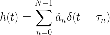
The complex channel response is given by

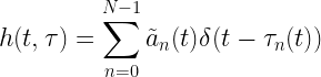
In the equation above, the attenuation and path delay vary with time. This simulates a time-variant complex channel.
As a special case, in the absence any movements or other changes in the transmission channel, the channel can remain fairly time invariant (fixed channel with respect to instantaneous time


Usually, the pair


propagation delays


Choose underlying distribution:
The next level of modeling involves, introduction of randomness in the above mentioned model there by rendering the channel response time variant. If the path attenuations are typically drawn from a complex Gaussian random variable, then at any given time


● Rayleigh distributed – if the mean of the distribution
● Rician distributed – if the mean of the distribution

![E [h(t; \tau)] = 0](https://s0.wp.com/latex.php?latex=E+%5Bh%28t%3B+%5Ctau%29%5D+%3D+0&bg=ffffff&fg=000&s=0&c=20201002)
![E [h(t; \tau)] \neq 0](https://s0.wp.com/latex.php?latex=E+%5Bh%28t%3B+%5Ctau%29%5D+%5Cneq+0&bg=ffffff&fg=000&s=0&c=20201002)
Respectively, these two scenarios model the presence or absence of a Line of Sight (LOS) path between the transmitter and the receiver. The first propagation delay


Similarly, the propagation delays can also be randomized, resulting in a more realistic but extremely complex model to implement. Furthermore, the power-delay-profile specifications with arbitrary time delays, warrant non-uniformly spaced tapped-delay-line filters, that are not suitable for practical simulation. For ease of implementation, the given PDP model with arbitrary time delays can be converted to tractable uniformly spaced statistical model by a combination of interpolation/approximation/uniform-sampling of the given power-delay-profile.
Real-life modelling:
Usually continuous domain equations for modeling multipath are specified in standards like COST-207 model in GSM specification. Such continuous time power-delay-profile models can be simulated using discrete-time Tapped Delay Line (TDL) filter with


Rate this article: Note: There is a rating embedded within this post, please visit this post to rate it.
References:
[1] Julius O. Smith III, Physical Audio Signal Processing, W3K Publishing, 2010, ISBN 978-0-9745607-2-4.↗
[2] M. Paetzold, A. Szczepanski, N. Youssef, Methods for Modeling of Specified and Measured Multipath Power-Delay Profiles, IEEE Trans. on Vehicular Techn., vol.51, no.5, pp.978-988, Sep.2002.↗
Topics in this chapter
| Small-scale Models for Multipath Effects ● Introduction ● Statistical characteristics of multipath channels □ Mutipath channel models □ Scattering function □ Power delay profile □ Doppler power spectrum □ Classification of small-scale fading ● Rayleigh and Rice processes □ Probability density function of amplitude □ Probability density function of frequency ● Modeling frequency flat channel ● Modeling frequency selective channel □ Method of equal distances (MED) to model specified power delay profiles □ Simulating a frequency selective channel using TDL model |
Books by the author
 Wireless Communication Systems in Matlab Second Edition(PDF) Note: There is a rating embedded within this post, please visit this post to rate it. |  Digital Modulations using Python (PDF ebook) Note: There is a rating embedded within this post, please visit this post to rate it. |  Digital Modulations using Matlab (PDF ebook) Note: There is a rating embedded within this post, please visit this post to rate it. |
| Hand-picked Best books on Communication Engineering Best books on Signal Processing |
||


![X[k] = \displaystyle{\sum_{n=0}^{N-1} x[n] e^{-j\frac{2 \pi}{N} k n}}](https://s0.wp.com/latex.php?latex=X%5Bk%5D+%3D+%5Cdisplaystyle%7B%5Csum_%7Bn%3D0%7D%5E%7BN-1%7D+x%5Bn%5D+e%5E%7B-j%5Cfrac%7B2+%5Cpi%7D%7BN%7D+k+n%7D%7D+&bg=ffffff&fg=000&s=1&c=20201002)

![\tilde{x}[n] = \displaystyle{ \frac{1}{N} \sum_{k=0}^{N-1} X[k] e^{j \frac{2 \pi}{N} kn}}](https://s0.wp.com/latex.php?latex=%5Ctilde%7Bx%7D%5Bn%5D+%3D+%5Cdisplaystyle%7B+%5Cfrac%7B1%7D%7BN%7D+%5Csum_%7Bk%3D0%7D%5E%7BN-1%7D+X%5Bk%5D+e%5E%7Bj+%5Cfrac%7B2+%5Cpi%7D%7BN%7D+kn%7D%7D+&bg=ffffff&fg=000&s=1&c=20201002)

![\boxed{ \displaystyle{\sum_{n=0}^{N-1} x[n] y^{\ast}[n] = \frac{1}{N} \sum_{k=0}^{N-1} X[k] Y^{\ast}[k]}}](https://s0.wp.com/latex.php?latex=%5Cboxed%7B+%5Cdisplaystyle%7B%5Csum_%7Bn%3D0%7D%5E%7BN-1%7D+x%5Bn%5D+y%5E%7B%5Cast%7D%5Bn%5D+%3D+%5Cfrac%7B1%7D%7BN%7D+%5Csum_%7Bk%3D0%7D%5E%7BN-1%7D+X%5Bk%5D+Y%5E%7B%5Cast%7D%5Bk%5D%7D%7D+&bg=ffffff&fg=000&s=1&c=20201002)


![\begin{aligned} \sum_{n=0}^{N-1} x[n] y^{\ast}[n] &= \sum_{n=0}^{N-1} x[n] \left(\frac{1}{N} \sum_{k=0}^{N-1} Y[k] e^{j\frac{2 \pi}{N} k n} \right )^\ast \\ &= \frac{1}{N}\sum_{n=0}^{N-1} x[n] \sum_{k=0}^{N-1} Y^\ast[k] e^{-j\frac{2 \pi}{N} k n} \\ &= \frac{1}{N} \sum_{k=0}^{N-1} Y^\ast[k] \cdot \sum_{n=0}^{N-1} x[n] e^{-j\frac{2 \pi}{N} k n} \\ &= \frac{1}{N} \sum_{k=0}^{N-1} X[k] Y^\ast[k] \end{aligned}](https://s0.wp.com/latex.php?latex=%5Cbegin%7Baligned%7D+%5Csum_%7Bn%3D0%7D%5E%7BN-1%7D+x%5Bn%5D+y%5E%7B%5Cast%7D%5Bn%5D+%26%3D+%5Csum_%7Bn%3D0%7D%5E%7BN-1%7D+x%5Bn%5D+%5Cleft%28%5Cfrac%7B1%7D%7BN%7D+%5Csum_%7Bk%3D0%7D%5E%7BN-1%7D+Y%5Bk%5D+e%5E%7Bj%5Cfrac%7B2+%5Cpi%7D%7BN%7D+k+n%7D+%5Cright+%29%5E%5Cast+%5C%5C+%26%3D+%5Cfrac%7B1%7D%7BN%7D%5Csum_%7Bn%3D0%7D%5E%7BN-1%7D+x%5Bn%5D+%5Csum_%7Bk%3D0%7D%5E%7BN-1%7D+Y%5E%5Cast%5Bk%5D+e%5E%7B-j%5Cfrac%7B2+%5Cpi%7D%7BN%7D+k+n%7D+%5C%5C+%26%3D+%5Cfrac%7B1%7D%7BN%7D+%5Csum_%7Bk%3D0%7D%5E%7BN-1%7D+Y%5E%5Cast%5Bk%5D+%5Ccdot+%5Csum_%7Bn%3D0%7D%5E%7BN-1%7D+x%5Bn%5D+e%5E%7B-j%5Cfrac%7B2+%5Cpi%7D%7BN%7D+k+n%7D+%5C%5C+%26%3D+%5Cfrac%7B1%7D%7BN%7D+%5Csum_%7Bk%3D0%7D%5E%7BN-1%7D+X%5Bk%5D+Y%5E%5Cast%5Bk%5D+%5Cend%7Baligned%7D+&bg=ffffff&fg=000&s=1&c=20201002)

![\displaystyle{\sum_{n=0}^{N-1} x[n] x^\ast[n] = \frac{1}{N} \sum_{k=0}^{N-1} X[k] X^{\ast}[k]}](https://s0.wp.com/latex.php?latex=%5Cdisplaystyle%7B%5Csum_%7Bn%3D0%7D%5E%7BN-1%7D+x%5Bn%5D+x%5E%5Cast%5Bn%5D+%3D+%5Cfrac%7B1%7D%7BN%7D+%5Csum_%7Bk%3D0%7D%5E%7BN-1%7D+X%5Bk%5D+X%5E%7B%5Cast%7D%5Bk%5D%7D+&bg=ffffff&fg=000&s=1&c=20201002)

![x[n] x^\ast[n] = |x[n]|^2](https://s0.wp.com/latex.php?latex=x%5Bn%5D+x%5E%5Cast%5Bn%5D+%3D+%7Cx%5Bn%5D%7C%5E2&bg=ffffff&fg=000&s=0&c=20201002)

![\boxed{ \displaystyle{\sum_{n=0}^{N-1} \left| x[n] \right|^2 = \frac{1}{N} \sum_{k=0}^{N-1} \left| X[k] \right|^2 }}](https://s0.wp.com/latex.php?latex=%5Cboxed%7B+%5Cdisplaystyle%7B%5Csum_%7Bn%3D0%7D%5E%7BN-1%7D+%5Cleft%7C+x%5Bn%5D+%5Cright%7C%5E2+%3D+%5Cfrac%7B1%7D%7BN%7D+%5Csum_%7Bk%3D0%7D%5E%7BN-1%7D+%5Cleft%7C+X%5Bk%5D+%5Cright%7C%5E2+%7D%7D++&bg=ffffff&fg=000&s=1&c=20201002)

![[x_0,x_1,\cdots,x_{N-1}]](https://s0.wp.com/latex.php?latex=%5Bx_0%2Cx_1%2C%5Ccdots%2Cx_%7BN-1%7D%5D&bg=ffffff&fg=000&s=0&c=20201002)

![\displaystyle{ x_{MS} = \frac{ |x_0|^2 + |x_1|^2 + \cdots + |x_{N-1}|^2}{N} = \frac{1}{N} \sum_{n=0}^{N-1} |x[n]|^2 }](https://s0.wp.com/latex.php?latex=%5Cdisplaystyle%7B+x_%7BMS%7D+%3D+%5Cfrac%7B+%7Cx_0%7C%5E2+%2B+%7Cx_1%7C%5E2+%2B+%5Ccdots+%2B+%7Cx_%7BN-1%7D%7C%5E2%7D%7BN%7D+%3D+%5Cfrac%7B1%7D%7BN%7D+%5Csum_%7Bn%3D0%7D%5E%7BN-1%7D+%7Cx%5Bn%5D%7C%5E2+%7D+&bg=ffffff&fg=000&s=1&c=20201002)

![\displaystyle{ x_{MS} : \quad \frac{1}{N} \sum_{n=0}^{N-1} |x[n]|^2 = \frac{1}{N^2} \sum_{k=0}^{N-1} \left| X[k] \right|^2}](https://s0.wp.com/latex.php?latex=%5Cdisplaystyle%7B+x_%7BMS%7D+%3A+%5Cquad+%5Cfrac%7B1%7D%7BN%7D+%5Csum_%7Bn%3D0%7D%5E%7BN-1%7D+%7Cx%5Bn%5D%7C%5E2+%3D+%5Cfrac%7B1%7D%7BN%5E2%7D+%5Csum_%7Bk%3D0%7D%5E%7BN-1%7D+%5Cleft%7C+X%5Bk%5D+%5Cright%7C%5E2%7D+&bg=ffffff&fg=000&s=1&c=20201002)

![\displaystyle{ x_{RMS} = \sqrt{\frac{ |x_0|^2 + |x_1|^2 + \cdots + |x_{N-1}|^2}{N}} = \sqrt{\frac{1}{N} \sum_{n=0}^{N-1} |x[n]|^2 }}](https://s0.wp.com/latex.php?latex=%5Cdisplaystyle%7B+x_%7BRMS%7D+%3D+%5Csqrt%7B%5Cfrac%7B+%7Cx_0%7C%5E2+%2B+%7Cx_1%7C%5E2+%2B+%5Ccdots+%2B+%7Cx_%7BN-1%7D%7C%5E2%7D%7BN%7D%7D+%3D+%5Csqrt%7B%5Cfrac%7B1%7D%7BN%7D+%5Csum_%7Bn%3D0%7D%5E%7BN-1%7D+%7Cx%5Bn%5D%7C%5E2+%7D%7D+&bg=ffffff&fg=000&s=1&c=20201002)

![\displaystyle{ x_{RMS}: \quad \sqrt{\frac{1}{N} \sum_{n=0}^{N-1} |x[n]|^2} = \sqrt{\frac{1}{N^2} \sum_{k=0}^{N-1} \left| X[k] \right|^2}}](https://s0.wp.com/latex.php?latex=%5Cdisplaystyle%7B+x_%7BRMS%7D%3A+%5Cquad+%5Csqrt%7B%5Cfrac%7B1%7D%7BN%7D+%5Csum_%7Bn%3D0%7D%5E%7BN-1%7D+%7Cx%5Bn%5D%7C%5E2%7D+%3D+%5Csqrt%7B%5Cfrac%7B1%7D%7BN%5E2%7D+%5Csum_%7Bk%3D0%7D%5E%7BN-1%7D+%5Cleft%7C+X%5Bk%5D+%5Cright%7C%5E2%7D%7D+&bg=ffffff&fg=000&s=1&c=20201002)

