Power delay profile (PDP) — multipath power vs delay

In one sentence: A power delay profile (PDP) is the average power $latex P(\tau)$ that a multipath channel delivers at each excess delay $latex \tau$; its mean and RMS width give you the delay spread, and the Fourier transform of the PDP tells you the coherence bandwidth, that is, how frequency-selective the channel is.

A radio signal rarely reaches the receiver along a single path. Reflections off buildings, ground and walls arrive later and weaker than the direct ray, so a transmitted pulse comes out smeared in time. The PDP summarizes that smear in one curve. Almost every practical decision that depends on multipath — whether you need an equalizer, how long the OFDM cyclic prefix must be, which 3GPP channel model to simulate — starts from it.

Want to play before you read? Open the power delay profile demo, choose a profile, and watch delay spread and coherence bandwidth move in opposite directions.

1. Professor: what a power delay profile is

Model the channel as a time-varying linear filter with complex baseband impulse response $latex h(t,\tau)$: the response observed at time $latex t$ to an impulse sent $latex \tau$ seconds earlier. For $latex L$ discrete paths this is

$latex \displaystyle h(t,\tau) = \sum_{k=0}^{L-1} \alpha_k(t)\,\delta(\tau-\tau_k) \qquad (1)$

where $latex \alpha_k(t)$ is the complex gain of the $latex k$-th path and $latex \tau_k$ is its excess delay (measured from the first arrival). The gains fluctuate rapidly with the receiver position because of constructive and destructive interference, so a single snapshot of $latex |h(t,\tau)|^2$ is not very informative. The power delay profile is its ensemble average:

$latex \displaystyle S(\tau) = P(\tau) = \mathrm{E}\left\{ |h(t,\tau)|^2 \right\} \qquad (2)$

For the discrete channel in (1) with uncorrelated path gains this becomes a set of powers $latex P_k = \mathrm{E}\{|\alpha_k|^2\}$ at delays $latex \tau_k$, which is what the stem plot in Figure 1 shows.

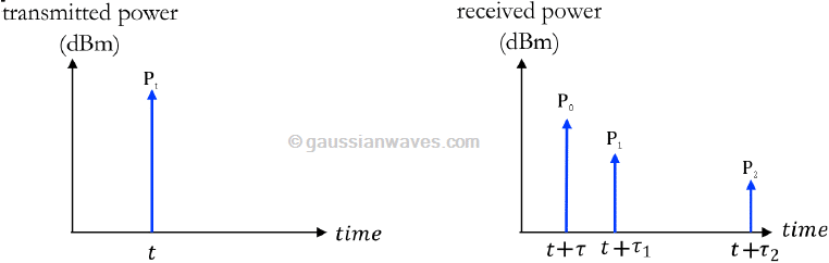
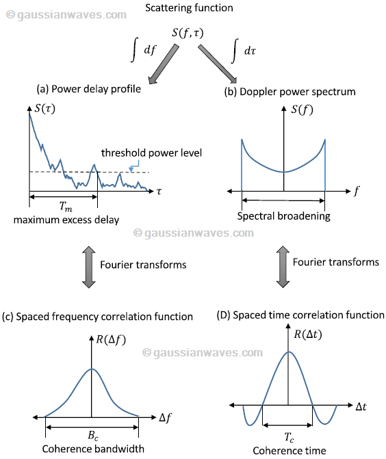
Professor’s note. The expectation in (2) is meaningful because of the wide-sense stationary uncorrelated scattering (WSSUS) assumption introduced by Bello [1]. “Wide-sense stationary” means the channel statistics depend only on the time difference $latex \Delta t$, not on absolute time. “Uncorrelated scattering” means that the gains arriving at different delays are uncorrelated, so $latex \mathrm{E}\{h(t,\tau)\,h^*(t+\Delta t,\tau’)\} = R_h(\Delta t,\tau)\,\delta(\tau-\tau’)$. Setting $latex \Delta t = 0$ gives exactly the PDP, $latex P(\tau) = R_h(0,\tau)$. Under WSSUS each delay bin is an independent Gaussian scatterer, which is why the taps of a TDL model can be generated independently. The PDP is the Doppler-integrated view of the scattering function: $latex P(\tau) = \int S(\tau,\nu)\,d\nu$.

2. Mean excess delay and RMS delay spread

Treat the normalized PDP $latex P(\tau)/\int P(\tau)\,d\tau$ as a probability density over delay. Its mean and standard deviation are the two numbers that characterize time dispersion. For a continuous PDP the mean excess delay and RMS delay spread are

$latex \displaystyle \mu_\tau = \frac{\int_{0}^{\infty} \tau\, P(\tau)\, d\tau}{\int_{0}^{\infty} P(\tau)\, d\tau} \qquad (3)$

$latex \displaystyle \sigma_\tau = \sqrt{\frac{\int_{0}^{\infty} (\tau-\mu_\tau)^2\, P(\tau)\, d\tau}{\int_{0}^{\infty} P(\tau)\, d\tau}} = \sqrt{\overline{\tau^2} – \mu_\tau^2} \qquad (4)$

For a discrete PDP with powers $latex P_k$ at delays $latex \tau_k$ the integrals become sums:

$latex \displaystyle \mu_\tau = \frac{\sum_k P_k\,\tau_k}{\sum_k P_k}, \qquad \sigma_\tau = \sqrt{\frac{\sum_k P_k\,(\tau_k-\mu_\tau)^2}{\sum_k P_k}} \qquad (5)$

Note that $latex \mu_\tau$ is a mean (no square root), and that dividing by the total power makes both statistics independent of how the PDP is scaled. A related number is the maximum excess delay $latex T_m$: the delay between the first arrival and the last component above a chosen threshold (for example 30 dB below the peak, or the receiver noise floor). It depends strongly on that threshold, whereas $latex \sigma_\tau$ is far more stable, which is one reason standards quote delay spread.

Two closed-form examples

Exponential PDP. The classic smooth-decay model is $latex P(\tau) = \frac{1}{\tau_{rms}}\, e^{-\tau/\tau_{rms}}$ for $latex \tau \ge 0$. Evaluating (3) and (4) gives $latex \mu_\tau = \sigma_\tau = \tau_{rms}$, so a single parameter sets everything.

Two-ray PDP. With powers $latex P_1, P_2$ at delays $latex 0$ and $latex \tau_2$, let $latex a = P_2/(P_1+P_2)$. Then $latex \mu_\tau = a\,\tau_2$ and

$latex \displaystyle \sigma_\tau = \tau_2\sqrt{a(1-a)} \qquad (6)$

which peaks at $latex \tau_2/2$ when the two rays have equal power. Try both in the demo and compare the readout with these formulas.

3. Coherence bandwidth: the frequency-domain twin

Delay dispersion in time is frequency selectivity in frequency. The channel’s frequency response is the Fourier transform of $latex h(t,\tau)$ over $latex \tau$, and its correlation between two frequencies separated by $latex \Delta f$ is the transform of the PDP:

$latex \displaystyle R_H(\Delta f) = \int_{0}^{\infty} P(\tau)\, e^{-j2\pi \Delta f \tau}\, d\tau \Big/ \int_{0}^{\infty} P(\tau)\, d\tau \qquad (7)$

The coherence bandwidth $latex B_c$ is the frequency separation over which $latex |R_H(\Delta f)|$ stays above a chosen level. Because it is the transform of the PDP, a wide PDP gives a narrow correlation and vice versa. Common rules of thumb are

$latex \displaystyle B_c \approx \frac{1}{5\,\sigma_\tau}\ (\text{correlation} \approx 0.5), \qquad B_c \approx \frac{1}{50\,\sigma_\tau}\ (\text{correlation} \approx 0.9), \qquad B_c \approx \frac{1}{2\pi\,\sigma_\tau} \qquad (8)$

For the exponential PDP the transform is exact: $latex |R_H(\Delta f)| = 1/\sqrt{1+(2\pi\,\Delta f\,\sigma_\tau)^2}$. That equals $latex 1/\sqrt 2 \approx 0.71$ at $latex \Delta f = 1/(2\pi\sigma_\tau)$, which is why the $latex 1/(2\pi\sigma_\tau)$ rule is the conservative one, and it equals $latex 0.5$ at $latex \Delta f = \sqrt 3/(2\pi\sigma_\tau) \approx 0.28/\sigma_\tau$, close to the $latex 1/(5\sigma_\tau)$ rule. The constants depend on the correlation level and on the PDP shape, but every rule has the same message: $latex B_c \propto 1/\sigma_\tau$. Double the delay spread and the coherence bandwidth halves.

Professor’s note. Rules of thumb are least reliable for PDPs that are not smooth. A two-ray channel has $latex |R_H(\Delta f)| = |\cos(\pi\,\Delta f\,\tau_2)|$ for equal powers: it is periodic with nulls every $latex 1/\tau_2$, so no single bandwidth describes it well. The demo reports the measured 0.5-correlation bandwidth next to the rules and marks the rules on the correlation plot, so you can see when they disagree.

4. Frequency-selective or flat?

The PDP lets you classify a link by comparing the channel with the signal. Let $latex W$ be the signal bandwidth and $latex T_{sym} \approx 1/W$ the symbol time.

• Flat (frequency-non-selective) fading: $latex W \ll B_c$, equivalently $latex \sigma_\tau \ll T_{sym}$. All frequencies in the signal fade together, the channel acts as a single complex gain, $latex y(t) = h(t)\,x(t) + w(t)$, and no equalizer is needed. A common practical guideline is $latex T_{sym} > 10\,\sigma_\tau$.
• Frequency-selective fading: $latex W \gtrsim B_c$, equivalently $latex \sigma_\tau$ comparable to or larger than $latex T_{sym}$. Echoes spill into neighbouring symbols (intersymbol interference) and different parts of the band fade differently, so the output is a convolution, $latex y(t) = \int h(t,\tau)\,x(t-\tau)\,d\tau + w(t)$. You need an equalizer, a RAKE receiver, or multicarrier modulation.

This is also why OFDM works so well on such channels: it splits the wide band into narrow subcarriers whose spacing is much smaller than $latex B_c$, so each subcarrier sees nearly flat fading, and a cyclic prefix longer than the significant echoes (roughly the maximum excess delay, or a few times $latex \sigma_\tau$) removes ISI entirely.

5. How a PDP is measured, and what the numbers look like

In the field the transmitter sends a wideband probe — a very short pulse, a pseudo-noise sequence correlated at the receiver, a chirp, or a swept tone measured with a network analyzer. The receiver records one complex impulse response $latex h(\tau)$ at each location. A single response is just one realization of the fading, so measurements are repeated over many positions within a small area (typically a few tens of wavelengths) and the squared magnitudes are averaged. That averaging is the empirical version of the expectation in (2). Three practical points matter:

• Delay resolution is about $latex 1/B_{probe}$. Paths closer than that merge into one tap, so a narrowband probe underestimates $latex \sigma_\tau$.
• Thresholding changes the answer. Noise adds a floor to every delay bin. Samples below a threshold set a few dB above the noise floor are discarded; otherwise the noise tail inflates $latex T_m$ and $latex \sigma_\tau$.
• Order of magnitude. Typical RMS delay spreads are on the order of tens of nanoseconds indoors, a few hundred nanoseconds in urban and suburban macrocells, and microseconds in hilly or long-range environments. Standards such as 3GPP specify short, nominal and long delay-spread variants of each model for this reason.

The resulting PDP is usually published as a table of delays and relative powers and serves as design guidance, not an exact description of any particular site. Maximum excess delay is also an input to positioning algorithms, and in early tapped-delay-line models such as CODIT [2] the number of FIR taps follows from the maximum excess delay times the sampling rate. The cyclic-prefix length of an OFDM system is likewise chosen from the maximum excess delay or the RMS delay spread of the target environment [3].

6. From a PDP to a simulation: TDL generation

A PDP is a statistical description; to simulate a link you need sample channel realizations. The tapped-delay-line (TDL) recipe turns a discrete PDP into a time-varying FIR filter:

1. List the delays $latex \tau_k$ and powers $latex P_k$ of the profile (rescale the delays to hit a target $latex \sigma_\tau$ if needed) and normalize $latex \sum_k P_k = 1$.
2. Resample the delays to the simulation sampling period $latex T_s$, merging taps that fall in the same sample bin.
3. For each tap draw an independent complex Gaussian process with variance $latex P_k$ and a Doppler spectrum (for example Jakes) matching the mobile speed. Under WSSUS these processes are independent, which is exactly what the PDP assumed.
4. Filter the transmit signal through $latex \sum_k \alpha_k(t)\,x(t-\tau_k)$ and add noise.

The detailed construction is in Modeling a frequency-selective multipath fading channel using TDL filters, and the 3GPP TDL channel calculator gives you the standardized delay and power tables together with the resulting delay spread and coherence bandwidth. Before you simulate, sanity-check the profile: the sample-domain PDP should reproduce the $latex \sigma_\tau$ you intended, which you can do with the same formulas in (5) or with the PDP demo.

Try it yourself

• Exponential PDP at 100 ns, pin it, then at 1 µs: $latex \sigma_\tau$ grows tenfold and $latex B_c$ shrinks to one tenth. Open the 1 µs case.
• Equal-power two-ray at 500 ns: $latex \sigma_\tau = 250$ ns and the correlation nulls every 2 MHz. Open it.
• Scale a custom tap table to a target delay spread and see which of your signal bandwidths becomes frequency-selective. Open it.

References

[1] P. A. Bello, Characterization of randomly time-variant linear channels, IEEE Trans. Comm. Syst., vol. 11, no. 4, pp. 360–393, Dec. 1963.
[2] P. G. Andermo and G. Larsson, Code division testbed, CODIT, 2nd International Conference on Universal Personal Communications, vol. 1, pp. 397–401, Oct. 1993.
[3] Huseyin Arslan, Cognitive Radio, Software Defined Radio, and Adaptive Wireless Systems, p. 238, Springer, 2007.

FAQ

What is a power delay profile in simple terms? It is a plot of the average received power against excess delay: how much of the transmitted pulse’s energy arrives right away, and how much arrives later via longer paths. Formally it is $latex \mathrm{E}\{|h(\tau)|^2\}$.

How is the PDP different from the channel impulse response? The impulse response $latex h(t,\tau)$ keeps complex amplitudes and phases and changes rapidly as you move; the PDP is its averaged squared magnitude, so it shows how power is spread over delay without the rapid phase detail.

What is the difference between mean excess delay and RMS delay spread? The mean excess delay $latex \mu_\tau$ is the centre of mass of the PDP; the RMS delay spread $latex \sigma_\tau$ is its standard deviation about that centre. Only $latex \sigma_\tau$ measures how smeared the pulse is, and only $latex \sigma_\tau$ enters the coherence-bandwidth rules.

How do I get coherence bandwidth from the delay spread? Use $latex B_c \approx 1/(5\sigma_\tau)$ for 0.5 correlation or $latex B_c \approx 1/(2\pi\sigma_\tau)$ for a conservative estimate, or transform the PDP as in (7) and read the frequency where $latex |R_H|$ crosses your chosen level. The demo shows all three.

Does normalizing the PDP change the delay spread? No. The moments in (3)–(5) divide by the total power, so only the relative powers matter.

How long should the OFDM cyclic prefix be? At least as long as the significant echoes, i.e. about the maximum excess delay of the environment above your threshold, which is typically several times $latex \sigma_\tau$. A longer prefix wastes rate; a shorter one leaves residual ISI.

How does the PDP connect to the 3GPP TDL models? Each TDL model is a normalized discrete PDP (delays and relative powers) plus a fading distribution per tap. Delays are scaled to the desired RMS delay spread. The 3GPP TDL channel calculator does that scaling and reports the resulting coherence bandwidth.

Similar articles

• Statistical characteristics of multipath channels: the scattering function
• Modeling a frequency-selective multipath fading channel using TDL filters
• Two-ray ground reflection model
• Orthogonality of OFDM