Compute signal power in Matlab

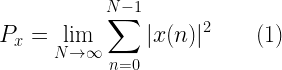
Calculating the energy and power of a signal was discussed in one of the previous posts. Here, we will verify the calculation of signal power using Discrete Fourier Transform (DFT) in Matlab. Check here to know more on the concept of power and energy.

The total power of a signal can be computed using the following equation

For other forms of equations: refer here.

This article is part of the following books
Digital Modulations using Matlab : Build Simulation Models from Scratch, ISBN: 978-1521493885
Digital Modulations using Python ISBN: 978-1712321638
Wireless communication systems in Matlab ISBN: 979-8648350779
All books available in ebook (PDF) and Paperback formats

Case Study:

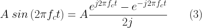
Let x(t) be a sine wave of amplitude A and frequency fc represented by the following equation.

When represented in frequency domain, it will look like the one on the right side plot in the following figure. This is evident from the fact that the sinewave can be mathematically represented by applying Euler’s formula.

Taking the Fourier transform of x(t) to represent it in frequency domain,

When considering the amplitude part,the above decomposition gives two spikes of amplitude A/2 on either side of the frequency domain at fc and -fc.

Figure 1: Time domain representation and frequency spectrum of a pure sinewave

Squaring the amplitudes gives the magnitude of power of the individual spikes/frequency components. The power spectrum is plotted below.

Figure 2: Power spectrum of a pure sinewave

Thus if the pure sinewave is of amplitude A=1V and frequency=100Hz, the power spectrum will have two spikes of value at 100 Hz and -100 Hz frequencies. The total power will be

Let’s verify this through simulation.

Simulation and Verification

A sine wave of 100 Hz frequency and amplitude 1V is taken for the experiment.

A=1; %Amplitude of sine wave
Fc=100; %Frequency of sine wave
Fs=1000; %Sampling rate - oversampled by the rate of 10
Ts=1/Fs; %Sampling period
nCycles=200; %Number of cycles of the sinewave

subplot(2,1,1);
t=0:Ts:nCycles/Fc-Ts; %Time base
x=A*sin(2*pi*Fc*t); %Sinusoidal function
stem(t,x); %Plot command

A sinusoidal wave of 10 cycles is plotted here

Figure 3: Sine wave generated in Matlab

Matlab’s Norm function:

Matlab’s basic installation comes with “norm” function. The p-norm in Matlab is computed as

By default, the single argument norm function computed 2-norm given as

To compute the total power of the signal x[n] (as in equation (1) above), all we have to do is – compute norm(x), square it and divide by the length of the signal.

L=length(x);
P=(norm(x)^2)/L;
sprintf('Power of the Signal from Time domain %f',P);

The above given piece of code will result in the following output

Power of the Signal from Time domain 0.500000

Verifying the total Power by DFT : Frequency Domain

Here, the total power is verified by applying DFT on the sinusoidal sequence. The sinusoidal sequence x[n] is represented in frequency domain X[f] using Matlab’s FFT function. The power associated with each frequency point is computed as

Finally, the total power is calculated as the sum of all the points in the frequency domain representation.

X = fft(x);
Px=sum(X.*conj(X))/(L^2); %Compute power with proper scaling.
subplot(2,1,2)
% Plot single-sided amplitude spectrum.
stem(Px);
sprintf('Total Power of the Signal from DFT %f',P);

Result:

Total Power of the Signal from DFT 0.500000
Figure 4: Power spectrum of a pure sinewave simulated in Matlab

A word on Matlab’s FFT: Matlab’s FFT is optimized for faster performance if the transform length is a power of 2. The following snippet of code simply calls “fft” without the transform length. In this case, the window length and the transform length are the same. This is to simplify the calculation of power. You can re-write the call to the FFT routine with transform length set to next power of two which is greater than or equal to the window length (sequence length). Then the step to compute total power will be differing slightly in the denominator. But that will not improve resolution (Remember : zero padding to compute FFT will not improve resolution).

Also note that in the above simulation we are using a pure sinusoid. The entire sequence of sinusoid defined all the cycles completely. There are no discontinuities in the sequence. If you call FFT with the transform length set to next power of 2 (as given in Matlab manuals), it will pad additional zeros to the sequence and creates discontinuities in the FFT computation. This will lead to spectral leakage. FFT and spectral leakage is discussed here.

Rate this article: Note: There is a rating embedded within this post, please visit this post to rate it.

References:

[1] Sanjay Lall,”Norm and Vector spaces”,Information Systems Laboratory,Stanford University.↗

Books by the author


Wireless Communication Systems in Matlab
Second Edition(PDF)

Note: There is a rating embedded within this post, please visit this post to rate it.
Checkout Added to cart

Digital Modulations using Python
(PDF ebook)

Note: There is a rating embedded within this post, please visit this post to rate it.
Checkout Added to cart
digital_modulations_using_matlab_book_cover
Digital Modulations using Matlab
(PDF ebook)

Note: There is a rating embedded within this post, please visit this post to rate it.
Checkout Added to cart
Hand-picked Best books on Communication Engineering
Best books on Signal Processing

Power and Energy of a Signal : Demystified

Key focus: Clearly understand the terms: power and energy of a signal, their mathematical definition, physical significance and computation in signal processing context.

Energy of a signal:

Defining the term “size”:

In signal processing, a signal is viewed as a function of time. The term “size of a signal” is used to represent “strength of the signal”. It is crucial to know the “size” of a signal used in a certain application. For example, we may be interested to know the amount of electricity needed to power a LCD monitor as opposed to a CRT monitor. Both of these applications are different and have different tolerances. Thus the amount of electricity driving these devices will also be different.

A given signal’s size can be measured in many ways. Given a mathematical function (or a signal equivalently), it seems that the area under the curve, described by the mathematical function, is a good measure of describing the size of a signal. A signal can have both positive and negative values. This may render areas that are negative. Due to this effect, it is possible that the computed values cancel each other totally or partially, rendering incorrect result. Thus the metric function of “area under the curve” is not suitable for defining the “size” of a signal. Now, we are left with two options : either 1) computation of the area under the absolute value of the function or 2) computation of the area under the square of the function. The second choice is favored due to its mathematical tractability and its similarity to Euclidean Norm which is used in signal detection techniques (Note: Euclidean norm – otherwise called L2 norm or 2-norm[1] – is often considered in signal detection techniques – on the assumption that it provides a reasonable measure of distance between two points on signal space. It is computed as Euclidean distance in detection theory).

This article is part of the following books
Digital Modulations using Matlab : Build Simulation Models from Scratch, ISBN: 978-1521493885
Digital Modulations using Python ISBN: 978-1712321638
Wireless communication systems in Matlab ISBN: 979-8648350779
All books available in ebook (PDF) and Paperback formats

Going by the second choice of viewing the “size” as the computation of the area under the square of the function, the energy of a continuous-time complex signal \(x(t)\) is defined as

\[E_x = \int_{-\infty}^{\infty} |x(t)|^2 dt\]

If the signal \(x(t)\) is real, the modulus operator in the above equation does not matter.

This is called “Energy” in signal processing terms. This is also a measure of signal strength. This definition can be applied to any signal (or a vector) irrespective of whether it possesses actual energy (a basic quantitative property as described by physics) or not. If the signal is associated with some physical energy, then the above definition gives the energy content in the signal. If the signal is an electrical signal, then the above definition gives the total energy of the signal (in Joules) dissipated over a 1 Ohm resistor.

Actual Energy – physical quantity:

To know the actual energy of the signal \(E\), one has to know the value of load \(Z\) the signal is driving and also the nature the electrical signal (voltage or current). For a voltage signal, the above equation has to be scaled by a factor of \(1/Z\).

\[E = \frac{E_x}{Z} = \frac{1}{Z} \int_{-\infty}^{\infty} |x(t)|^2 dt \]

For current signal, it has to be scaled by \(Z\).

\[E = ZE_x = Z \int_{-\infty}^{\infty} |x(t)|^2 dt\]

Here, \(Z\) is the impedance driven by the signal \(x(t)\) , \(E_x\) is the signal energy (signal processing term) and \(E\) is the Energy of the signal (physical quantity) driving the load \( Z\)

Energy in discrete domain:

In the discrete domain, the energy of the signal is given by

\[E_x = \displaystyle{ \sum_{n=-\infty}^{\infty} |x(n)|^2}\]

The energy is finite only if the above sum converges to a finite value. This implies that the signal is “squarely-summable“. Such a signal is called finite energy signal.

What if the given signal does not decay with respect to time (as in a continuous sine wave repeating its cycle infinitely) ? The energy will be infinite  and such a signal is “not squarely-summable” in other words. We need another measurable quantity to circumvent this problem.This leads us to the notion of “Power”

Power:

Power is defined as the amount of energy consumed per unit time. This quantity is useful if the energy of the signal goes to infinity or the signal is “not-squarely-summable”. For “non-squarely-summable” signals, the power calculated by taking the snapshot of the signal over a specific interval of time as follows

1) Take a snapshot of the signal over some finite time duration
2) Compute the energy of the signal \(E_x\)
3) Divide the energy by number of samples taken for computation \(N\)
4) Extend the limit of number of samples to infinity \(N\rightarrow \infty \). This gives the total power of the signal.

In discrete domain, the total power of the signal is given by

\[P_x = \lim_{N \rightarrow \infty } \frac{1}{2N+1} \displaystyle{\sum_{n=-N}^{n=+N} |x(n)|^2} \]

Following equations are different forms of the same computation found in many text books. The only difference is the number of samples taken for computation. The denominator changes according to the number of samples taken for computation.

\[\begin{align} P_x &= \lim_{N \rightarrow \infty } \frac{1}{2N} \displaystyle{\sum_{n=-N}^{n=N-1} |x(n)|^2} \\ P_x &= \lim_{N \rightarrow \infty } \frac{1}{N} \displaystyle{\sum_{n=0}^{n=N-1} |x(n)|^2} \\ P_x &= \lim_{N \rightarrow \infty } \frac{1}{N_1 – N_0 + 1} \displaystyle{\sum_{n=N_0}^{n=N_1} |x(n)|^2} \end{align} \]

Classification of Signals:

A signal can be classified based on its power or energy content. Signals having finite energy are energy signals. Power signals have finite and non-zero power.

Energy Signal :

A finite energy signal will have zero TOTAL power. Let’s investigate this statement in detail. When the energy is finite, the total power will be zero. Check out the denominator in the equation for calculating the total power. When the limit \(N\rightarrow \infty\), the energy dilutes to zero over the infinite duration and hence the total power becomes zero.

Power Signal:

Signals whose total power is finite and non-zero. The energy of the power signal will be infinite. Example: Periodic sequences like sinusoid. A sinusoidal signal has finite, non-zero power but infinite energy.

A signal cannot be both an energy signal and a power signal.

Neither an Energy signal nor a Power signal:

Signals can also be a cat on the wall – neither an energy signal nor a power signal. Consider a signal of increasing amplitude defined by,

\[x(n) = n\]

For such a signal, both the energy and power will be infinite. Thus, it cannot be classified either as an energy signal or as a power signal.

Calculation of power and verifying it through Matlab is discussed next…

Rate this article: Note: There is a rating embedded within this post, please visit this post to rate it.

References:

[1] Sanjay Lall,”Norm and Vector spaces”,Information Systems Laboratory,Stanford University.↗

Books by the author


Wireless Communication Systems in Matlab
Second Edition(PDF)

Note: There is a rating embedded within this post, please visit this post to rate it.
Checkout Added to cart

Digital Modulations using Python
(PDF ebook)

Note: There is a rating embedded within this post, please visit this post to rate it.
Checkout Added to cart

Digital Modulations using Matlab
(PDF ebook)

Note: There is a rating embedded within this post, please visit this post to rate it.
Checkout Added to cart
Hand-picked Best books on Communication Engineering
Best books on Signal Processing

Similar Topics

Essentials of Signal Processing
● Generating standard test signals
 □ Sinusoidal signals
 □ Square wave
 □ Rectangular pulse
 □ Gaussian pulse
 □ Chirp signal
Interpreting FFT results - complex DFT, frequency bins and FFTShift
 □ Real and complex DFT
 □ Fast Fourier Transform (FFT)
 □ Interpreting the FFT results
 □ FFTShift
 □ IFFTShift
Obtaining magnitude and phase information from FFT
 □ Discrete-time domain representation
 □ Representing the signal in frequency domain using FFT
 □ Reconstructing the time domain signal from the frequency domain samples
● Power spectral density
Power and energy of a signal
 □ Energy of a signal
 □ Power of a signal
 □ Classification of signals
 □ Computation of power of a signal - simulation and verification
Polynomials, convolution and Toeplitz matrices
 □ Polynomial functions
 □ Representing single variable polynomial functions
 □ Multiplication of polynomials and linear convolution
 □ Toeplitz matrix and convolution
Methods to compute convolution
 □ Method 1: Brute-force method
 □ Method 2: Using Toeplitz matrix
 □ Method 3: Using FFT to compute convolution
 □ Miscellaneous methods
Analytic signal and its applications
 □ Analytic signal and Fourier transform
 □ Extracting instantaneous amplitude, phase, frequency
 □ Phase demodulation using Hilbert transform
Choosing a filter : FIR or IIR : understanding the design perspective
 □ Design specification
 □ General considerations in design