Key focus: How to implement the basic addition operation on two discrete time signal sequences. Python code for signal addition is provided.
Signal addition
Given two discrete-time sequences \(x_1[n]\) and \(x_2[n]\), the addition of these two sequences is represented as \(x_1[n]+ x_2[n]\). The start of the sample at \(n=0\) can be different for these two sequences.
the position of the sample at \(n=0\) is different in these sequences. Also, the length of these sequences are different.
The addition operation should take these differences into account. The following python code adjusts for these differences before computing the addition operation. It creates two sequences y1[n]y1[n] and y2[n]y2[n] of equal length that spans the minimum and maximum indices of x1[n]x1[n] and x2[n]x2[n]. The sequences y1[n]y1[n] and y2[n]y2[n] are first filled with zeros and then the sequences x1[n]x1[n] & x2[n]x2[n] are copied over to y1[n]y1[n] & y2[n]y2[n] at corresponding positions. The final result is computed as the sum of y1[n]y1[n] and y2[n]y2[n].
import numpy as np

def signal_add(x1, n1, x2, n2):
    '''
    Computes y(n) = x1(n) + x2(n)
    ---------------------------------
    [y, n] = signal_add(x1, n1, x2, n2)

    Parameters
    ----------
    n1 = indices of first sequence x1
    n2 = indices of second sequence x2
    x1 = first sequence defined for indices n1
    x2 = second sequence defined for indices n2
    Returns
    -------
    y = output sequence defined over indices n that
    covers whole range of n1 and n2
    '''

    n_start = min(min(n1), min(n2))
    n_end = max(max(n1), max(n2))
    n = np.arange(n_start, n_end + 1)  # duration of y(n)

    y1 = np.zeros_like(n, dtype='complex_')
    y2 = np.zeros_like(n, dtype='complex_')

    mask1 = (n >= n1[0]) & (n <= n1[-1])
    mask2 = (n >= n2[0]) & (n <= n2[-1])

    y1[np.where(mask1)[0]] = x1[np.where(n1 == n[mask1])]
    y2[np.where(mask2)[0]] = x2[np.where(n2 == n[mask2])]

    y = y1 + y2

    return y, n
The following code snippet uses the function above to compute the addition of two sequences \(x_1[n]\) and \(x_2[n]\), defined as
\[\begin{align} x_1[n] &= cos \left( 0.03 \pi n \right), & 0 \leq n \leq 50 \\ x_2[n] &= e^{0.06 n}, & -30 \leq 0 \leq n \end{align}\]
In digital signal processing, we utilize various elementary sequences for the purpose of analysis. In this series, we will see such sequences. One such elementary sequence is the real-valued exponential sequence. (see the articles on unit sample sequence, unit step sequence, real-valued exponential sequence)
A complex-valued exponential sequence in signals and systems is a discrete-time sequence that exhibits complex exponential behavior. It is characterized by complex numbers raised to the power of the index. The general form of a complex-valued exponential sequence is given by:
\[x[n] = e^{ \alpha n }e^{ j \omega n } = e^{\left( \alpha + j \omega \right) n } = cos \left[ \left( \alpha + j \omega \right) n \right] + j sin \left[ \left( \alpha + j \omega \right) n \right], \; \forall n \]
where:
x[n] is the value of the sequence at index n.
\(\alpha\) acts as an attenuation factor if \(\alpha \lt 0\) or as an amplification factor for \(\alpha \gt 0\)
\(j\) is the indeterminate satisfying \(j^2 = -1\) (imaginary unit).
\(\omega\) is the angular frequency in radians per sample.
The complex nature is indicated by the presence of the indeterminate \(j\) in the exponent.
The python function to generate a complex exponential function is given below
import numpy as np
import matplotlib.pyplot as plt

def complex_exponential_sequence(n, alpha, omega):
    return  np.exp((alpha + 1j * omega) * n)

n = np.linspace(0, 40, 1000)
alpha = 0.025; omega = 0.75
x = complex_exponential_sequence(n, alpha, omega)
Plot of real and imaginary parts of the sequence generated for various values of \(\alpha\) and \(\omega\) is given next
Figure 1: Complex exponential sequence for various values of \(\alpha\) and \(\omega\)
From Figure 1, we see that the variable \(\alpha\) governs the decay or growth of the sequence in time and the \(\omega\) controls the oscillation frequency on a circle in the complex plane.
The 3D views of the complex sequence for various values of \(\alpha\) and \(\omega\) are illustrated next.
When (\(\alpha=0\)), the sequence remains the on circle in the complex plane.
Figure 2: A neutral sequence (\(\alpha =0\) and \(\omega = 1\))
When \(\alpha \gt 0 \), the sequence grows exponentially and it spirals out.
Figure 3: A growing sequence (\(\alpha >0\) and \(\omega = 0.75 \))
When \(\alpha \lt 0 \), the sequence decays exponentially.
Figure 4: A decaying sequence (\(\alpha <0\) and \(\omega = 2.5 \))
Applications
Complex exponential sequences have various applications in modeling and signal processing. Some of the key applications include:
Signal Analysis and Representation: Complex exponential sequences form the basis for Fourier analysis, which decomposes a signal into a sum of sinusoidal components. The complex exponential sequence (\(e^{j\omega n}\)) serves as the building block for representing and analyzing signals in the frequency domain.
System Modeling and Analysis: These sequences play a fundamental role in modeling and analyzing linear time-invariant (LTI) systems. By applying complex exponential inputs to a system and observing the resulting outputs, one can determine the system’s frequency response and characterize its behavior in terms of amplitude and phase shifts at different frequencies.
Digital Filtering: Complex exponential sequences are utilized in digital filtering algorithms, such as the Fourier transform-based frequency domain filtering and the Z-transform-based discrete-time filtering. These sequences help design filters for various applications, such as noise removal, equalization, and signal enhancement.
Modulation Techniques: These sequences are fundamental in various modulation schemes used in communication systems. For instance, in amplitude modulation (AM), frequency modulation (FM), and phase modulation (PM), the modulating signals are typically expressed as complex exponential sequences that are mixed with carrier signals to encode information.
Control Systems: Complex exponential sequences are relevant in control system analysis and design. In control theory, the Laplace transform, which involves complex exponentials, is used to analyze system dynamics, stability, and transient response. The concept of the complex plane, where complex exponentials reside, is crucial in control system design and stability analysis.
Digital Signal Processing (DSP): These sequences find extensive use in various DSP applications, including digital audio processing, image processing, speech recognition, and data compression. Techniques like the discrete Fourier transform (DFT) and fast Fourier transform (FFT) exploit complex exponentials to efficiently analyze signals in the frequency domain.
In digital signal processing, we utilize various elementary sequences for the purpose of analysis. In this series, we will see such sequences. One such elementary sequence is the real-valued exponential sequence. (see the articles on unit sample sequence, unit step sequence, complex exponential sequence)
An exponential sequence in signals and systems is a discrete-time sequence that exhibits exponential growth or decay. It is characterized by a constant base raised to the power of the index. The general form of the sequence is given by:
\[x[n] = A \cdot r^n, \quad \forall n; \quad r \in \mathbb{R}\]
where:
\(x[n]\) is the value of the sequence at index \(n\).
\(A\) is the initial amplitude or value at \(n = 0\).
\(r\) is the constant base, which determines the growth or decay behavior.
\(n\) represents the index of the sequence.
If the value of r is greater than 1, the sequence grows exponentially as n increases, resulting in exponential growth. Conversely, if r is between 0 and 1, the sequence decays exponentially, approaching zero as n increases.
Exponential sequences find various applications in fields such as finance, physics, and telecommunications. In signal processing and system analysis, these sequences are fundamental components used to model and analyze various system behaviors, such as stability, convergence, and frequency response.
Python code that implements a real-valued exponential sequence for various values of \(r\).
import matplotlib.pyplot as plt
import numpy as np

def exponential_sequence(n, A, r):
    return A * np.power(r, n)

# Define the range of n
n = np.arange(0, 25)

# Define the values of r
r_values = [0.5, 0.8, 1.2]

# Plotting the exponential sequences for various values of r
fig, axs = plt.subplots(len(r_values), 1, figsize=(8, 6))

for i, r in enumerate(r_values):
    # Generate the exponential sequence for the current value of r
    x = exponential_sequence(n, 1, r)

    # Plot the exponential sequence in the current subplot
    axs[i].stem(n, x, 'k', use_line_collection=True)
    axs[i].set_xlabel('n')
    axs[i].set_ylabel(f'x[n], r={r}')
    axs[i].set_title(f'Exponential Sequence, r={r}')
    axs[i].grid(True)

# Adjust spacing between subplots
plt.tight_layout()

# Display the plot
plt.show()
Figure 1: Real-valued exponential sequence \(x[n] = A \cdot r^n\) for \(r = 0.5, 0.8, 1.5\)
Applications
Real-valued exponential sequences have various applications in different fields, including:
Signal Processing: Exponential sequences are used to model and analyze signals in fields like audio processing, image processing, and telecommunications. They are fundamental in Fourier analysis, frequency response analysis, and filter design.
System Analysis: Exponential sequences are essential in understanding and characterizing the behavior of linear time-invariant (LTI) systems. They help analyze system stability, impulse response, and frequency response.
Finance: Exponential sequences find applications in finance and economics for modeling compound interest, population growth, investment returns, and other exponential growth/decay phenomena.
Physics: In physics, exponential sequences are used to describe natural phenomena such as radioactive decay, charging/discharging of capacitors, and decay of electrical or mechanical systems.
Control Systems: Exponential sequences play a crucial role in control systems engineering. They are used to model system dynamics, analyze stability, and design controllers for desired response characteristics.
Probability and Statistics: Exponential sequences are utilized in probability and statistics to model various distributions, including the exponential distribution, which represents events occurring randomly and independently over time.
Machine Learning: Exponential sequences are used in machine learning algorithms for tasks such as feature scaling, regularization, and gradient descent optimization.
These are just a few examples of the broad range of applications where real-valued exponential sequences are utilized. Their ability to represent exponential growth or decay makes them a valuable tool for modeling and understanding dynamic systems and phenomena in various disciplines.
In digital signal processing, we utilize various elementary sequences for the purpose of analysis. In this series, we will see such sequences. One such elementary sequence is the unit step sequence (see the articles on unit sample sequence, unit step sequence, real-valued exponential sequence, complex exponential sequence).
Unit Step Sequence
A unit step sequence is a discrete-time signal that represents a step function. In discrete-time signal processing, a sequence is a set of values indexed by integers. A unit step sequence, denoted as u[n], is defined as follows:
In this definition, the value of \(u[n]\) is 0 for negative values of \(n\) (\(n \lt 0\)), and it is 1 for non-negative values of \(n (n \geq 0)\). The up-arrow indicates the sample at \(n=0\)
Graphically, the sequence looks like a step function, where the value remains zero for negative indices and abruptly jumps to 1 at n=0, continuing at that value for positive indices.
In the equation above, the sequence value of 1 start at index 0. In signal processing, the starting place (where the value 1 starts) can be shifted. The generalized formula for generated a shifted sequence will be
\[ u[n – n_0] = \begin{cases} 1 , & \quad n \geq n_0 \\ 0, & \quad n \lt n_0\end{cases}\]
The following python code implements a unit step sequence over the interval \(n_1 \leq n \leq n_2\)
import matplotlib.pyplot as plt
import numpy as np

def unit_step_sequence(n0, n1, n2):
    """
    Generate unit step sequence u(n - n0); n1<=n<=n
    n0 = number of samples to offset/shift
    n1 = starting number to generate the sequence index
    n2 = ending number to generate the sequence index
    """
    n = np.arange(n1,n2+1)
    u = np.zeros_like(n)
    u[n >= n0] = 1
    return u

# Generate the shifted unit step sequence for a given range and shift value
n0 = 2  # Shift value
n1 = -3
n2 = 9
u = unit_step_sequence(n0, n1, n2)

fig = plt.figure()
ax = fig.add_subplot(1, 1, 1)

# Plotting the shifted unit step sequence
plt.stem(np.arange(n1,n2+1), u,'r', markerfmt='o', basefmt='k', use_line_collection=True)
plt.xlabel('n')
plt.ylabel(r'$u[n-n_0]$')
plt.title(r'Discrete-time Unit Step Sequence $u[n-2]$')
plt.grid(True)
plt.show()
Figure 1: Discrete unit step sequence \(u[n-n_0]\); shifted by \(n_0=2\), generated over the interval \(-3 <= n <= 9\)
Applications
The unit step sequence is often used as a fundamental building block in signal processing and system analysis. It serves as a basic reference for studying and analyzing other signals and systems. By manipulating the sequence, one can derive other useful sequences and functions, such as shifted step sequences, ramp sequences, and more complex signals.
This sequence is particularly important in the field of discrete-time systems, where it is used to analyze system behavior and characterize properties like stability, causality, and linearity. It is also employed in various applications, such as digital filters, signal modeling, and signal reconstruction.
In digital signal processing, we utilize various elementary sequences for the purpose of analysis. In this series, we will see such sequences. One such elementary sequence is the unit sample sequence (see the articles on unit sample sequence, unit step sequence, real-valued exponential sequence, complex exponential sequence)
A unit sample sequence, also known as an impulse sequence or delta sequence, is a discrete sequence that consists of a single sample with the value of 1 at a specific index, and all other samples are zero. It is commonly represented as a discrete-time impulse function or delta function.
Mathematically, a unit sample sequence can be defined as:
\(x[n]\) represents the value of the sequence at index \(n\).
\(δ[n]\) is the discrete-time impulse function or delta function.
\(n_0\) is the index at which the impulse occurs. At this index, \(x[n]\) has the value of 1, and for all other indices, \(x[n]\) is zero.
This sequence represents a localized impulse or sudden change at that particular index. The unit sample sequence is commonly used in signal processing and system analysis to study the response of systems to impulses or abrupt changes. It serves as a fundamental tool for representing and analyzing signals and systems.
In python, the scipy.signal.unit_impulse function can be used to generate an impulse sequence in SciPy. For 1-D signals, the first argument to the function is the number of samples requested for generating the unit_impulse and the second argument is the offset (i.e, \(n_0\))
import matplotlib.pyplot as plt
import numpy as np
from scipy import signal

n = 11 #number of samples
n0 = 5 # Offset (Shift index)
imp = signal.unit_impulse(n, n0) #unit impulse

fig = plt.figure()
ax = fig.add_subplot(1, 1, 1)

plt.stem(np.arange(0,n),imp,'r', markerfmt='ro', basefmt='k')
plt.xlabel('Sample #')
plt.ylabel(r'$\delta[n-n_0]$')
plt.title('Discrete-time Unit Impulse')
plt.show()
Figure 1: Discrete-time unit impulse
Applications of unit sample sequences
Unit sample sequences, also known as impulse sequences, have several applications in digital signal processing. Here are a few common applications:
System Analysis: Unit sample sequences are used to analyze and characterize the behavior of systems, such as filters and signal processors, in response to impulses or sudden changes.
Convolution: Unit sample sequences are essential in the mathematical operation of convolution, which is used for filtering, signal analysis, and processing tasks.
Signal Reconstruction: Unit sample sequences are employed in reconstructing continuous signals from their sampled versions using techniques like impulse sampling and interpolation.
System Identification: Unit sample sequences can be utilized to estimate the impulse response of a system, allowing for system identification and modeling.
These are just a few examples of the diverse applications of unit sample sequences in digital signal processing. They serve as fundamental tools for analyzing signals, characterizing systems, and performing various signal processing operations.
In the context of signal and systems, analog and discrete signals are two different types of signals that convey information.
Analog signal
An analog signal is a continuous signal that varies smoothly over time. It can take on any value within a certain range. Analog signals are represented by physical quantities such as voltage, current, or sound waves. For example, the varying voltage produced by a microphone when recording sound is an analog signal. Analog signals are typically represented as continuous waveforms.
Let’s consider an example of a simple analog signal:
\[x(t) = A \cdot sin \left(2 \pi f t + \phi \right)\]
In this equation:
x(t) represents the value of the analog signal at time t.
A is the amplitude of the signal, which determines its maximum value.
f is the frequency of the signal, which represents the number of cycles per unit of time.
φ is the phase of the signal, which represents the offset or starting point of the waveform.
This equation describes a sinusoidal analog signal, where the value of the signal varies continuously over time. The signal can have an infinite number of values at any given instant.
Discrete signal
On the other hand, a discrete signal is a signal that is defined only at specific instances of time and takes on a finite set of values. Discrete signals are often derived from analog signals by a process called sampling, where the continuous analog signal is measured or sampled at regular intervals. Each sample represents the value of the signal at a particular instant. These samples can be stored and processed using digital systems. Examples of discrete signals include digital audio, digital images, and the output of a digital sensor.
Discrete signals are commonly used in digital signal processing and can be represented using mathematical equations.
The general equation for a discrete signal can be written as:
\[x[n] = f(n)\]
In this equation:
x[n] represents the value of the discrete signal at time instance n.
f(n) is the function that determines the value of the signal at each specific time instance.
The function f(n) can take various forms depending on the specific characteristics of the discrete signal. For example, let’s start with the equation for the analog sinusoidal signal:
\[x(t) = A \cdot sin \left(2 \pi f t + \phi \right)\]
To obtain the discrete version of this signal, we need to sample it at regular intervals. The sampling process involves measuring the analog signal at equidistant points in time.
Let’s define the sampling period as \(T_s\), which represents the time between two consecutive samples. The sampling rate is the inverse of the sampling period and is denoted as \(f_s = 1 / T_s\).
Now, we can express the discrete version of the sinusoidal signal as:
\[x[n] = x(n T_s) = A \cdot sin(2 \pi f n T_s + \phi)\]
In this equation:
x[n] represents the value of the discrete signal at sample index n.
f is the frequency of the sinusoidal signal in hertz
n represents the sample index, indicating which sample we are considering.
\(T_s\) is the sampling period.
\(f_s\) is the sampling frequency, which is the reciprocal of the sampling period.
By substituting \(nT_s\) for t in the analog sinusoidal signal equation, we obtain the discrete version of the sinusoidal signal. The discrete signal represents the sampled values of the original analog signal at each specific time instance, \(nT_s\).
It’s important to note that the accuracy of the discrete signal representation depends on the sampling rate. According to the Nyquist-Shannon sampling theorem, for real signals, the sampling rate should be at least twice the maximum frequency of the analog signal to avoid aliasing and accurately reconstruct the signal from its samples.
Python code
Following is an example Python code that simulates an analog sinusoidal signal, samples it to obtain a discrete version, and overlays the two signals for comparison
import numpy as np
import matplotlib.pyplot as plt

# Parameters for the analog signal
amplitude = 1.0  # Amplitude of the signal
frequency = 2.0  # Frequency of the signal in Hz
phase = 0.0  # Phase of the signal in radians

# Parameters for the discrete signal
sampling_rate = 10  # Number of samples per second
num_samples = 20

# Time arrays for the analog and discrete signals
t_analog = np.linspace(0, num_samples / sampling_rate, num_samples * 10)  # Higher resolution for analog signal
n_discrete = np.arange(num_samples)

# Generate the analog signal
analog_signal = amplitude * np.sin(2 * np.pi * frequency * t_analog + phase)

# Sample the analog signal to obtain the discrete signal
discrete_signal = amplitude * np.sin(2 * np.pi * frequency * n_discrete / sampling_rate + phase)

# Plot the analog and discrete signals
plt.plot(t_analog, analog_signal, label='Analog Signal')
plt.stem(n_discrete / sampling_rate, discrete_signal, 'r', markerfmt='ro', basefmt=' ', label='Discrete Signal')
plt.xlabel('Time')
plt.ylabel('Amplitude')
plt.title('Analog and Discrete Sinusoidal Signals')
# Move the legend outside the figure
plt.legend(loc='upper right', bbox_to_anchor=(1.1, 1))
plt.grid(True)
plt.show()
Resulting plot
Figure 1: Simulated analog and discrete sinusoidal signals
Orthogonality is a mathematical principle that signifies the absence of correlation or relationship between two vectors (signals). It implies that the vectors or signals involved are mutually independent or unrelated.
Two vectors (signals) A and B are said to be orthogonal (perpendicular in vector algebra) when their inner product (also known as dot product) is zero.
To find the dot product of two vectors, you need to multiply their corresponding components and then sum the results. Here’s the general formula (in matrix notation) for checking the orthogonality of two complex valued vectors \(\vec{a}\) and \(\vec{b}\):
Here’s an example code snippet in Python that demonstrates to check if two vectors given as lists are orthogonal.
import numpy as np
import matplotlib.pyplot as plt

def dot_product(vector1, vector2):
    if len(vector1) != len(vector2):
        raise ValueError("Vectors must have the same length.")
    return sum(x * y for x, y in zip(vector1, vector2))

def are_orthogonal(vector1, vector2):
    result = dot_product(vector1, vector2)
    return result == 0

# Example vectors
vectorA = [-2, 3]
vectorB = [3, 2]

# Check if vectors are orthogonal
if are_orthogonal(vectorA, vectorB):
    print("The vectors are orthogonal.")
else:
    print("The vectors are not orthogonal.")

# Plotting the vectors
origin = [0], [0]  # Origin point for the vectors

plt.quiver(*origin, vectorA[0], vectorA[1], angles='xy', scale_units='xy', scale=1, color='r', label='Vector A')
plt.quiver(*origin, vectorB[0], vectorB[1], angles='xy', scale_units='xy', scale=1, color='b', label='Vector B')

plt.xlim(-5, 5)
plt.ylim(-5, 5)
plt.xlabel('x')
plt.ylabel('y')
plt.title('Plot of Vectors')
plt.grid(True)
plt.legend()
plt.show()
Orthogonality of Continuous functions
Orthogonality, in the context of functions, can be seen as a broader concept akin to the orthogonality observed in vectors. Geometrically, orthogonal vectors are perpendicular to each other since their dot product equals zero.
When computing the dot product of two vectors, their components are multiplied and summed. However, when considering the “dot” product of functions, a similar approach is taken. Functions are treated as if they were vectors with an infinite number of components, and the dot product is obtained by multiplying the functions together and integrating over a specific interval.
Let f(t) and g(t) are two continuous functions (imagined as two vectors) on the closed interval [a,b] (i.e a ≤ t ≤ b). For the functions to be orthogonal in the given interval, their dot product should be zero
\[ \left<f,g\right> = \int_a^b f(t) g(t) dt = 0 \Rightarrow \text{f(t) and g(t) are orthogonal}\]
Here is a small python script to check if two given functions are orthogonal
Python Script
import sympy
import numpy as np
import matplotlib.pyplot as plt

plt.style.use('seaborn-talk')
print(plt.style.available)

# Test the orthogonality of functions
x = sympy.Symbol('x')
f = sympy.sin(x)  # First function
g = sympy.cos(2*x)  # Second function
a = 0 # interval lower limit
b = 2*sympy.pi # interval upper limit
interval = (0, 2*sympy.pi)  # Integration interval
inner_product = sympy.integrate(f*g, (x, interval[0], interval[1]))

if sympy.N(inner_product) == 0:
    print("The functions",str(f),"and",str(g),"are orthogonal over the interval [",str(a), ",",str(b),"].")
else:
    print("The functions",str(f),"and",str(g),"are not orthogonal over the interval [",str(a), ",",str(b),"].")

# Plotting the functions
x_vals = np.linspace(float(interval[0]), float(interval[1]), 100)
f_vals = np.sin(x_vals)
g_vals = np.cos(2*x_vals)

plt.plot(x_vals, f_vals, label=str(f))
plt.plot(x_vals, g_vals, label=str(g))
plt.plot(x_vals, f_vals*g_vals, label=str(f)+str(g))
plt.xlabel('x')
plt.ylabel('Function values')
plt.legend()
plt.title('Plot of functions')
plt.grid(True)
plt.show()
Output
The functions sin(x) and cos(2*x) are orthogonal over the interval [ 0 , 2*pi ]
Orthogonality of discrete functions
To check the orthogonality of discrete functions, you can use the concept of the inner product (same as above). In discrete settings, the inner product can be thought of as the sum of the element-wise products of the function values at corresponding points.
Here’s an example code snippet in Python that demonstrates how to check the orthogonality of two discrete functions:
import numpy as np

def inner_product(f, g):
    if len(f) != len(g):
        raise ValueError("Functions must have the same length.")
    return np.sum(f * g)

def are_orthogonal(f, g):
    result = inner_product(f, g)
    return result == 0

# Example functions (discrete)
f = np.array([1, 0, -1, 0])
g = np.array([0, 1, 0, -1])

# Check if functions are orthogonal
if are_orthogonal(f, g):
    print("The functions are orthogonal.")
else:
    print("The functions are not orthogonal.")
Since you have landed on this page, probably you are looking for an opportunity to write for this website. I assume that you have looked around and you know that I take this website seriously. I am committed to adding value to my readers and to you as an author.
I am currently accepting guest posts from sincere and credible readers like you. You do not need to have a great content to start with. You can even share what you have learned about a fascinating concept.
You can go here directly and start writing your post. Be sure to login before writing the post
Guidelines
Your post must be original and not previously published either on the Web or in print.
You can include images (must not be copyrighted or copied from some other websites) in your post
You agree not to publish it anywhere else, including your own blog or Web site. You may, however, post a brief summary on your site that links to the post.
You may provide up to three byline links: one for your blog or Web site, one for your bio or About page, and one for your Linkedin URL.
Your post should be at least 300 words long and no more than 800 words.
You must register yourself as a member on this website: To do so, just login here with the list of available social network login option
You must have a profile picture of yourself. As you as you log in your profile picture from the social network will be automatically used. You can change this any time.
Your articles can fall into any of the following categories:
Research article (empirical-quantitative and qualitative- and/or theoretical)
Research note/Tutorials
Blog posts on a particular topic
Code snippets (Matlab,python,C,C++ etc..,) – tips and tricks
Book reviews
Project reports
Your articles can be in the field of electrical/electronics/communication/computer engineering discipline. The intended discipline spans a wide range of sub-disciplines such as signal processing, communications, electronics design, applied mathematics for signal processing, biomedical signal processing, Image processing etc., You could also choose a specific list of disciplines , some example listed below.
Multichannel & multimodal signal processing
Audio/Speech processing
Biomedical signal processing
Image/multimedia processing
Analog Communications
Digital communications
Implementation, design, and hardware for signal processing/communications
Statistical signal processing
Random process and Probability
Applied mathematics related to electrical/electronics/communication/computer engineering
Electronic Circuits
VLSI/embedded/etc..,
Editing
I will likely redact your post for grammar, punctuation, spelling, etc. If I make substantive changes (unlikely), I will email the post back to you for your approval before posting.
Responding to comments
Please confirm that you are willing to engage with my readers in the comments about your post. This is hugely important and a non-negotiable. My readers have come to expect this. You may need to login in the comment section using a disqus account for this.
Submission
If your post meets the above guidelines, please go ahead write post in the form given below. Alternatively, you can also send your post as MS DOC to mathuranathanv@gmail.com
Once your content is finalized, I will publish your articles under your name. At anytime, you can populate your social media profiles for Facebook, Twitter, LinkedIn, Google+ and your Author Bio for your account. Make sure you are happy with the details about your author profile.
We live in the age of smart phones that can be loaded with numerous applications to communicate with each other. What’s next ? Where do we go from here ?
Students at MIT Media Labs has answered the call with a novel approach of “Physical Telepresence” that provides the ability to remotely render shapes of objects and people.
Physical telepresence is the result of InFORM interface invented at MIT Media Labs. InForm interface is a self-aware interface, that manipulates not only light but also shapes as well. With this new technology, two remotely connected people can interact with each other by playing a ball game, manipulating shapes/objects together etc..,
This website uses cookies to improve your experience while you navigate through the website. Out of these, the cookies that are categorized as necessary are stored on your browser as they are essential for the working of basic functionalities of the website. We also use third-party cookies that help us analyze and understand how you use this website. These cookies will be stored in your browser only with your consent. You also have the option to opt-out of these cookies. But opting out of some of these cookies may affect your browsing experience.
Necessary cookies are absolutely essential for the website to function properly. These cookies ensure basic functionalities and security features of the website, anonymously.
Cookie
Duration
Description
cookielawinfo-checbox-analytics
11 months
This cookie is set by GDPR Cookie Consent plugin. The cookie is used to store the user consent for the cookies in the category "Analytics".
cookielawinfo-checbox-analytics
11 months
This cookie is set by GDPR Cookie Consent plugin. The cookie is used to store the user consent for the cookies in the category "Analytics".
cookielawinfo-checbox-functional
11 months
The cookie is set by GDPR cookie consent to record the user consent for the cookies in the category "Functional".
cookielawinfo-checbox-functional
11 months
The cookie is set by GDPR cookie consent to record the user consent for the cookies in the category "Functional".
cookielawinfo-checbox-others
11 months
This cookie is set by GDPR Cookie Consent plugin. The cookie is used to store the user consent for the cookies in the category "Other.
cookielawinfo-checbox-others
11 months
This cookie is set by GDPR Cookie Consent plugin. The cookie is used to store the user consent for the cookies in the category "Other.
cookielawinfo-checkbox-necessary
11 months
This cookie is set by GDPR Cookie Consent plugin. The cookies is used to store the user consent for the cookies in the category "Necessary".
cookielawinfo-checkbox-performance
11 months
This cookie is set by GDPR Cookie Consent plugin. The cookie is used to store the user consent for the cookies in the category "Performance".
viewed_cookie_policy
11 months
The cookie is set by the GDPR Cookie Consent plugin and is used to store whether or not user has consented to the use of cookies. It does not store any personal data.
Functional cookies help to perform certain functionalities like sharing the content of the website on social media platforms, collect feedbacks, and other third-party features.
Performance cookies are used to understand and analyze the key performance indexes of the website which helps in delivering a better user experience for the visitors.
Analytical cookies are used to understand how visitors interact with the website. These cookies help provide information on metrics the number of visitors, bounce rate, traffic source, etc.