In digital signal processing, we utilize various elementary sequences for the purpose of analysis. In this series, we will see such sequences. One such elementary sequence is the unit sample sequence (see the articles on unit sample sequence, unit step sequence, real-valued exponential sequence, complex exponential sequence)
A unit sample sequence, also known as an impulse sequence or delta sequence, is a discrete sequence that consists of a single sample with the value of 1 at a specific index, and all other samples are zero. It is commonly represented as a discrete-time impulse function or delta function.
Mathematically, a unit sample sequence can be defined as:
\[x[n] = \delta[n – n_0] = \begin{cases} 1 & \quad n = n_0 \\ 0 & \quad n \neq n_0 \end{cases} \]Where:
- \(x[n]\) represents the value of the sequence at index \(n\).
- \(δ[n]\) is the discrete-time impulse function or delta function.
- \(n_0\) is the index at which the impulse occurs. At this index, \(x[n]\) has the value of 1, and for all other indices, \(x[n]\) is zero.
This sequence represents a localized impulse or sudden change at that particular index. The unit sample sequence is commonly used in signal processing and system analysis to study the response of systems to impulses or abrupt changes. It serves as a fundamental tool for representing and analyzing signals and systems.
In python, the scipy.signal.unit_impulse function can be used to generate an impulse sequence in SciPy. For 1-D signals, the first argument to the function is the number of samples requested for generating the unit_impulse and the second argument is the offset (i.e, \(n_0\))
import matplotlib.pyplot as plt
import numpy as np
from scipy import signal

n = 11 #number of samples
n0 = 5 # Offset (Shift index)
imp = signal.unit_impulse(n, n0) #unit impulse

fig = plt.figure()
ax = fig.add_subplot(1, 1, 1)

plt.stem(np.arange(0,n),imp,'r', markerfmt='ro', basefmt='k')
plt.xlabel('Sample #')
plt.ylabel(r'$\delta[n-n_0]$')
plt.title('Discrete-time Unit Impulse')
plt.show()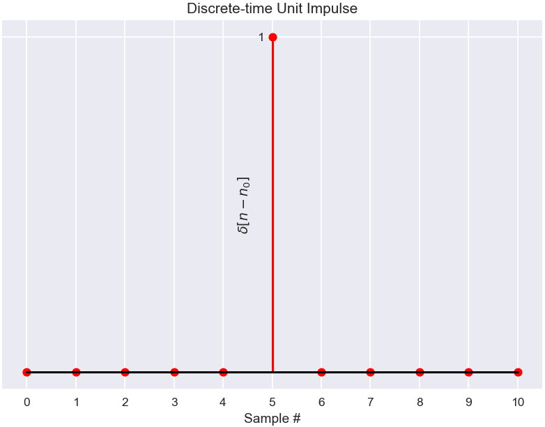
Applications of unit sample sequences
Unit sample sequences, also known as impulse sequences, have several applications in digital signal processing. Here are a few common applications:
System Analysis: Unit sample sequences are used to analyze and characterize the behavior of systems, such as filters and signal processors, in response to impulses or sudden changes.
Convolution: Unit sample sequences are essential in the mathematical operation of convolution, which is used for filtering, signal analysis, and processing tasks.
Signal Reconstruction: Unit sample sequences are employed in reconstructing continuous signals from their sampled versions using techniques like impulse sampling and interpolation.
System Identification: Unit sample sequences can be utilized to estimate the impulse response of a system, allowing for system identification and modeling.
These are just a few examples of the diverse applications of unit sample sequences in digital signal processing. They serve as fundamental tools for analyzing signals, characterizing systems, and performing various signal processing operations.