Keywords: orthogonality, vectors, functions, dot product, inner product, discrete, Python programming, data analysis, visualization
This post contains interactive python code which you can execute in the browser itself.
Orthogonality
Orthogonality is a mathematical principle that signifies the absence of correlation or relationship between two vectors (signals). It implies that the vectors or signals involved are mutually independent or unrelated.
Two vectors (signals) A and B are said to be orthogonal (perpendicular in vector algebra) when their inner product (also known as dot product) is zero.
$$A \perp B \Leftrightarrow \left<A.B \right> = A_1 \cdot B_1 + A_2 \cdot B_2 + \cdots A_n \cdot B_n = 0$$
Example: Let’s show that the two vectors \(\overrightarrow{A} = \binom{-2}{3}\) and \(\overrightarrow{B} = \binom{3}{2}\) are orthogonal
\[\overrightarrow{A} \cdot \overrightarrow{B} = A_x B_x + A_y B_y = (-2)(3) + (3)(2) = 0 \]Let verify if the angle between the vectors is \(90^{\circ}\)
\[ \theta = cos^{-1} \left( \frac{\overrightarrow{A} \cdot \overrightarrow{B}}{|\overrightarrow{A} | |\overrightarrow{B}|} \right) = cos^{-1}(0) = 90 ^{\circ} \]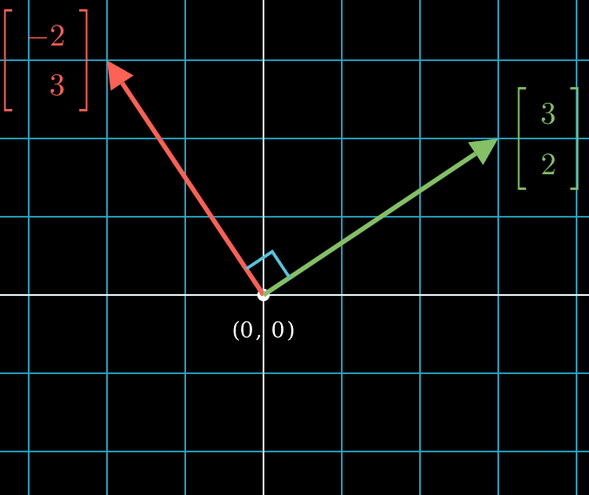
To find the dot product of two vectors, you need to multiply their corresponding components and then sum the results. Here’s the general formula (in matrix notation) for checking the orthogonality of two complex valued vectors \(\vec{a}\) and \(\vec{b}\):
$$\vec{a} \perp \vec{b} \Rightarrow \left< \vec{a}, \vec{b} \right> = \begin{bmatrix} a_1^* & a_2^* & \cdots & a_n^* \ \end{bmatrix} \begin{bmatrix}b_1 \\b_2\\\vdots \\b_n \end{bmatrix} = 0$$
Here’s an example code snippet in Python that demonstrates to check if two vectors given as lists are orthogonal.
import numpy as np
import matplotlib.pyplot as plt

def dot_product(vector1, vector2):
    if len(vector1) != len(vector2):
        raise ValueError("Vectors must have the same length.")
    return sum(x * y for x, y in zip(vector1, vector2))

def are_orthogonal(vector1, vector2):
    result = dot_product(vector1, vector2)
    return result == 0

# Example vectors
vectorA = [-2, 3]
vectorB = [3, 2]

# Check if vectors are orthogonal
if are_orthogonal(vectorA, vectorB):
    print("The vectors are orthogonal.")
else:
    print("The vectors are not orthogonal.")

# Plotting the vectors
origin = [0], [0]  # Origin point for the vectors

plt.quiver(*origin, vectorA[0], vectorA[1], angles='xy', scale_units='xy', scale=1, color='r', label='Vector A')
plt.quiver(*origin, vectorB[0], vectorB[1], angles='xy', scale_units='xy', scale=1, color='b', label='Vector B')

plt.xlim(-5, 5)
plt.ylim(-5, 5)
plt.xlabel('x')
plt.ylabel('y')
plt.title('Plot of Vectors')
plt.grid(True)
plt.legend()
plt.show()
Orthogonality of Continuous functions
Orthogonality, in the context of functions, can be seen as a broader concept akin to the orthogonality observed in vectors. Geometrically, orthogonal vectors are perpendicular to each other since their dot product equals zero.
When computing the dot product of two vectors, their components are multiplied and summed. However, when considering the “dot” product of functions, a similar approach is taken. Functions are treated as if they were vectors with an infinite number of components, and the dot product is obtained by multiplying the functions together and integrating over a specific interval.
Let f(t) and g(t) are two continuous functions (imagined as two vectors) on the closed interval [a,b] (i.e a ≤ t ≤ b). For the functions to be orthogonal in the given interval, their dot product should be zero
$$\left<f,g\right> = \int_a^b f(t) g(t) dt = 0 \Rightarrow \text{f(t) and g(t) are orthogonal}$$
Here is a small python script to check if two given functions are orthogonal
Interactive Python Script
Simulation Result:
Reference result:
The functions sin(x) and cos(2*x) are orthogonal over the interval [ 0 , 2*pi ]

Orthogonality of discrete functions
To check the orthogonality of discrete functions, you can use the concept of the inner product (same as above). In discrete settings, the inner product can be thought of as the sum of the element-wise products of the function values at corresponding points.
Here’s an example code snippet in Python that demonstrates how to check the orthogonality of two discrete functions:
import numpy as np

def inner_product(f, g):
    if len(f) != len(g):
        raise ValueError("Functions must have the same length.")
    return np.sum(f * g)

def are_orthogonal(f, g):
    result = inner_product(f, g)
    return result == 0

# Example functions (discrete)
f = np.array([1, 0, -1, 0])
g = np.array([0, 1, 0, -1])

# Check if functions are orthogonal
if are_orthogonal(f, g):
    print("The functions are orthogonal.")
else:
    print("The functions are not orthogonal.")