Analog vs discrete signals — continuous time, sampling, and sequences

In one sentence: Analog signals are defined for a continuum of time; discrete-time signals are sequences $latex x[n]$ — usually samples of an analog waveform under a sampling theorem constraint.

In the context of signal and systems, analog and discrete signals are two different types of signals that convey information.

This post contains interactive python code which you can execute in the browser itself.

Analog signal

An analog signal is a continuous signal that varies smoothly over time. It can take on any value within a certain range. Analog signals are represented by physical quantities such as voltage, current, or sound waves. For example, the varying voltage produced by a microphone when recording sound is an analog signal. Analog signals are typically represented as continuous waveforms.

Let’s consider an example of a simple analog signal:

$$ x(t) = A \cdot sin \left(2 \pi f t + \phi \right)$$

In this equation:

• x(t) represents the value of the analog signal at time t.
• A is the amplitude of the signal, which determines its maximum value.
• f is the frequency of the signal, which represents the number of cycles per unit of time.
• φ is the phase of the signal, which represents the offset or starting point of the waveform.

This equation describes a sinusoidal analog signal, where the value of the signal varies continuously over time. The signal can have an infinite number of values at any given instant.

Discrete signal

On the other hand, a discrete signal is a signal that is defined only at specific instances of time and takes on a finite set of values. Discrete signals are often derived from analog signals by a process called sampling, where the continuous analog signal is measured or sampled at regular intervals. Each sample represents the value of the signal at a particular instant. These samples can be stored and processed using digital systems. Examples of discrete signals include digital audio, digital images, and the output of a digital sensor.

Discrete signals are commonly used in digital signal processing and can be represented using mathematical equations.

The general equation for a discrete signal can be written as:

$$x[n] = f(n)$$

In this equation:

• x[n] represents the value of the discrete signal at time instance n.
• f(n) is the function that determines the value of the signal at each specific time instance.

The function f(n) can take various forms depending on the specific characteristics of the discrete signal. For example, let’s start with the equation for the analog sinusoidal signal:

$$x(t) = A \cdot sin \left(2 \pi f t + \phi \right$$

To obtain the discrete version of this signal, we need to sample it at regular intervals. The sampling process involves measuring the analog signal at equidistant points in time.

Let’s define the sampling period as$latex T_s$, which represents the time between two consecutive samples. The sampling rate is the inverse of the sampling period and is denoted as$latex f_s = 1 / T_s$.

Now, we can express the discrete version of the sinusoidal signal as:

$$x[n] = x(n T_s) = A \cdot sin(2 \pi f n T_s + \phi)$$

In this equation:

• x[n] represents the value of the discrete signal at sample index n.
• f is the frequency of the sinusoidal signal in hertz
• n represents the sample index, indicating which sample we are considering.
• $latex T_s$ is the sampling period.
• $latex f_s$ is the sampling frequency, which is the reciprocal of the sampling period.

By substituting$latex nT_s$ for t in the analog sinusoidal signal equation, we obtain the discrete version of the sinusoidal signal. The discrete signal represents the sampled values of the original analog signal at each specific time instance,$latex nT_s$.

It’s important to note that the accuracy of the discrete signal representation depends on the sampling rate. According to the Nyquist-Shannon sampling theorem, for real signals, the sampling rate should be at least twice the maximum frequency of the analog signal to avoid aliasing and accurately reconstruct the signal from its samples.

Python code

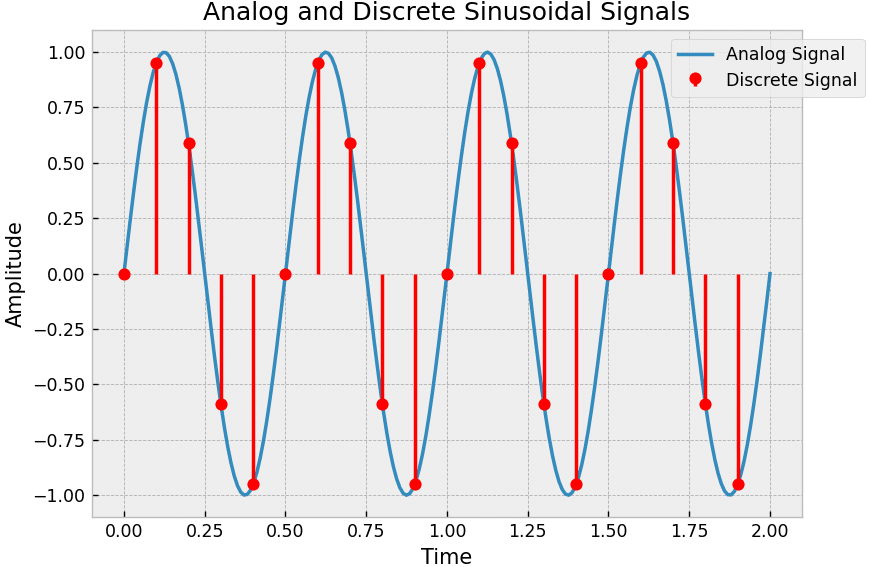
Following is an example Python code that simulates an analog sinusoidal signal, samples it to obtain a discrete version, and overlays the two signals for comparison.

Simulated Result:

Reference plot

FAQ

What is the difference between a discrete-time signal and a digital signal? Discrete-time means the signal is defined only on integer indices $latex n$ (a sequence). Digital usually also implies quantized amplitudes. You can have discrete-time real-valued sequences in analysis long before quantization is introduced.

How do we convert an analog waveform into a discrete-time sequence? Uniform sampling after an anti-alias filter, with the rate chosen by the Nyquist theorem for the signal’s bandwidth. The sampling article in this lab path covers the aliasing constraints in detail.

Do energy and power formulas change between analog and discrete time? Yes in appearance: continuous-time energy uses $latex \int|x(t)|^2\,dt$; discrete-time energy uses $latex \sum|x[n]|^2$ (sometimes scaled by the sample period $latex T_s$ to keep physical units). The concepts — accumulate $|x|^2$ — stay the same.

Similar articles

• Sampling theorem
• Power and energy
• Unit step sequence