Binomial random variable using Matlab

Binomial random variable, a discrete random variable, models the number of successes in mutually independent Bernoulli trials, each with success probability . The term Bernoulli trial implies that each trial is a random experiment with exactly two possible outcomes: success and failure. It can be used to model the total number of bit errors in the received data sequence of length that was transmitted over a binary symmetric channel of bit-error probability .

Generating binomial random sequence in Matlab

Let X denotes the total number of successes in mutually independent Bernoulli trials. For ease of understanding, let’s denote success as ‘1’ and failure as ‘0’. Suppose if a particular outcome of the experiment contains ones and zeros (example outcome: 1011101), the probability mass function↗ of is given by

A binomial random variable can be simulated by generating independent Bernoulli trials and summing up the results.

function X = binomialRV(n,p,L)
%Generate Binomial random number sequence
%n - the number of independent Bernoulli trials
%p - probability of success yielded by each trial
%L - length of sequence to generate
X = zeros(1,L);
for i=1:L,
   X(i) = sum(bernoulliRV(n,p));
end
end

Following program demonstrates how to generate a sequence of binomially distributed random numbers, plot the estimated and theoretical probability mass functions for the chosen parameters (Figure 1).

n=30; p=1/6; %number of trails and success probability
X = binomialRV(n,p,10000);%generate 10000 bino rand numbers
X_pdf = pdf('Binomial',0:n,n,p); %theoretical probility density
histogram(X,'Normalization','pdf'); %plot histogram
hold on; plot(0:n,X_pdf,'r'); %plot computed theoreical PDF
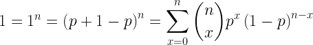
PMF generated from binomial random variable for three different cases of n and p
Figure 1: PMF generated from binomial random variable for three different cases of n and p

PMF sums to unity

Let’s verify theoretically, the fact that the PMF of the binomial distribution sums to unity. Using the result of Binomial theorem↗,

Mean and variance

The mean number of success in a binomial distribution is

The variance is

Rate this article: Note: There is a rating embedded within this post, please visit this post to rate it.

Topics in this chapter

Random Variables - Simulating Probabilistic Systems
● Introduction
Plotting the estimated PDF
● Univariate random variables
 □ Uniform random variable
 □ Bernoulli random variable
 □ Binomial random variable
 □ Exponential random variable
 □ Poisson process
 □ Gaussian random variable
 □ Chi-squared random variable
 □ Non-central Chi-Squared random variable
 □ Chi distributed random variable
 □ Rayleigh random variable
 □ Ricean random variable
 □ Nakagami-m distributed random variable
Central limit theorem - a demonstration
● Generating correlated random variables
 □ Generating two sequences of correlated random variables
 □ Generating multiple sequences of correlated random variables using Cholesky decomposition
Generating correlated Gaussian sequences
 □ Spectral factorization method
 □ Auto-Regressive (AR) model

Books by the author


Wireless Communication Systems in Matlab
Second Edition(PDF)

Note: There is a rating embedded within this post, please visit this post to rate it.
Checkout Added to cart

Digital Modulations using Python
(PDF ebook)

Note: There is a rating embedded within this post, please visit this post to rate it.
Checkout Added to cart

Digital Modulations using Matlab
(PDF ebook)

Note: There is a rating embedded within this post, please visit this post to rate it.
Checkout Added to cart
Hand-picked Best books on Communication Engineering
Best books on Signal Processing

Bernoulli random variable

Bernoulli random variable is a discrete random variable with two outcomes – success and failure, with probabilities p and (1-p). It is a good model for binary data generators and also for modeling bit error patterns in the received binary data when a communication channel introduces random errors.

To generate a Bernoulli random variable X, in which the probability of success P(X=1)=p for some p ϵ (0,1), the discrete inverse transform method [1] can be applied on the continuous uniform random variable U(0,1) using the steps below.

  ● Generate uniform random number U in the interval (0,1)
  ● If U<p, set X=1, else set X=0

#bernoulliRV.m: Generating Bernoulli random number with success probability p
function X = bernoulliRV(L,p)
%Generate Bernoulli random number with success probability p
%L is the length of the sequence generated
U = rand(1,L); %continuous uniform random numbers in (0,1)
X = (U<p); end

Verifying law of large numbers

In probability theory, the law of large numbers is a theorem that involves repeating an experiment for a large number of times. According to this law, as the number of trials tend to become large, the average result obtained will be close to the expected value.

This article is part of the book
Wireless Communication Systems in Matlab (second edition), ISBN: 979-8648350779 available in ebook (PDF) format and Paperback (hardcopy) format.

Let’s toss a coin with probability of heads . This experiment is repeated for a large number of times, say and the average result for each trial are calculated in a cumulative fashion.

#lawOfLargeNumbers.m: Law of large numbers illustrated using Bernoulli random variable
n=1000; %number of trials
p=0.7; %probability of success
X=bernoulliRV(n,p); %Bernoulli random variable
y_sum=sum(triu(repmat(X,[prod(size(X)) 1])')); %cumulative sum
avg = y_sum./(1:1:n); %average of results
plot(1:1:n,avg,'.'); hold on;
xlabel('Trial #'); ylabel('Probability of Heads');
plot(p*ones(1,n),'r'); legend('average','expected');

Refer the book Wireless Communication Systems in Matlab for full Matlab code

Figure 1: Illustrating law of large numbers using Bernoulli trials

The resulting plot (Figure 1) shows that as the number of trial increases, the average approaches the expected value 0.7.

Rate this article: Note: There is a rating embedded within this post, please visit this post to rate it.

References

[1] L. Devroye, Non-Uniform Random Variate Generation, Springer-Verlag, New York, 1986.↗

Books by the author


Wireless Communication Systems in Matlab
Second Edition(PDF)

Note: There is a rating embedded within this post, please visit this post to rate it.
Checkout Added to cart

Digital Modulations using Python
(PDF ebook)

Note: There is a rating embedded within this post, please visit this post to rate it.
Checkout Added to cart

Digital Modulations using Matlab
(PDF ebook)

Note: There is a rating embedded within this post, please visit this post to rate it.
Checkout Added to cart
Hand-picked Best books on Communication Engineering
Best books on Signal Processing

Topics in this chapter

Random Variables - Simulating Probabilistic Systems
● Introduction
Plotting the estimated PDF
● Univariate random variables
 □ Uniform random variable
 □ Bernoulli random variable
 □ Binomial random variable
 □ Exponential random variable
 □ Poisson process
 □ Gaussian random variable
 □ Chi-squared random variable
 □ Non-central Chi-Squared random variable
 □ Chi distributed random variable
 □ Rayleigh random variable
 □ Ricean random variable
 □ Nakagami-m distributed random variable
Central limit theorem - a demonstration
● Generating correlated random variables
 □ Generating two sequences of correlated random variables
 □ Generating multiple sequences of correlated random variables using Cholesky decomposition
Generating correlated Gaussian sequences
 □ Spectral factorization method
 □ Auto-Regressive (AR) model