In the previous post, a method for generating two sequences of correlated random variables was discussed. Generation of multiple sequences of correlated random variables, given a correlation matrix is discussed here.
Correlation Matrix
Correlation matrix defines correlation among N variables. It is a symmetric $latex N \times N$ matrix with the $latex (ij)^{th}$ element equal to the correlation coefficient $latex r_{ij} $ between the $latex i^{th}$ and the $latex j^{th}$ variable. The diagonal elements (correlations of variables with themselves) are always equal to 1.
Sample problem:
Let’s say we would like to generate three sets of random sequences X,Y,Z with the following correlation relationships.
- Correlation co-efficient between X and Y is 0.5
- Correlation co-efficient between X and Z is 0.3
- Obviously the variable X correlates with itself 100% – i.e, correlation-coefficient is 1
Putting all these relationships in a compact matrix form, gives the correlation matrix. We take arbitrary correlation value (0.3) for the relationship between Y and Z.
$latex \bordermatrix{ & X & Y & Z \cr X & 1 & -0.5 & .3 \cr Y & -0.5 & 1 & .2 \cr Z & .3 & .2 & 1 } &s=2$
Now, the task is to generate three sets of random numbers X,Y and Z that follows the relationship above. The problem can be addressed in many ways. Two most common methods finding the solution are
- Cholesky Decomposition method
- Spectral Decomposition ( also called Eigen Vector Decomposition) method
The Cholesky Decomposition method is discussed here.
[table “36” not found /]
Generating Correlated random number using Cholesky Decomposition:
Cholesky decomposition is the matrix equivalent of taking square root operation on a given matrix. As with any scalar values, positive square root is only possible if the given number is a positive (Imaginary roots do exist otherwise). Similarly, if a matrix need to be decomposed into square-root equivalent, the matrix need to be positive definite.
The method discussed here, seeks to decompose the given correlation matrix using Cholesky decomposition.
$latex C = U^TU = LL^T &s=2$
where U and L are upper and lower triangular matrices. We will consider Upper triangular matrix here. Equivalently, lower triangular matrix can also be used, in which case the order of output needs to be reversed.
$latex C = U^TU &s=2$
For this decomposition to work, the correlation matrix should be positive definite. The correlated random sequences $latex R_c=[X,Y, Z]$ (where X,Y,Z are column vectors) that follow the above relationship can be generated by multiplying the uncorrelated random numbers R with U .
$latex R_c = RU &s=2$
Steps to follow:
Generate three sequences of uncorrelated random numbers R – each drawn from a normal distribution. For this case, the R matrix will be of size $latex k \times 3$ where k is the number of samples we wish to generate and we allocate the k samples in three columns, where the columns indicate the place holder for each variable X, Y and Z. Multiply this matrix with the Cholesky decomposed upper triangular version of the correlation matrix.
Python code
import numpy as np
from scipy.linalg import cholesky
from scipy.stats import pearsonr #to calculate correlation coefficient

#for plotting and visualization
import pandas as pd
import matplotlib.pyplot as plt
%matplotlib inline
plt.style.use('fivethirtyeight')
import seaborn as sns

C = np.array([[1, -0.5, 0.3],
              [-0.5, 1, 0.2],
              [0.3, 0.2, 1]]) #Construct correlation matrix
U = cholesky(C) #Cholesky decomposition
R = np.random.randn(10000,3) #Three uncorrelated sequences
Rc = R @ U #Array of correlated random sequences

#compute and display correlation coeff from generated sequences
def pearsonCorr(x, y, **kws):
    (r, _) = pearsonr(x, y) #returns Pearson’s correlation coefficient, 2-tailed p-value)
    ax = plt.gca()
    ax.annotate("r = {:.2f} ".format(r),xy=(.7, .9), xycoords=ax.transAxes)

#Visualization
df = pd.DataFrame(data=Rc, columns=['X','Y','Z'])
graph = sns.pairplot(df)
graph.map(pearsonCorr)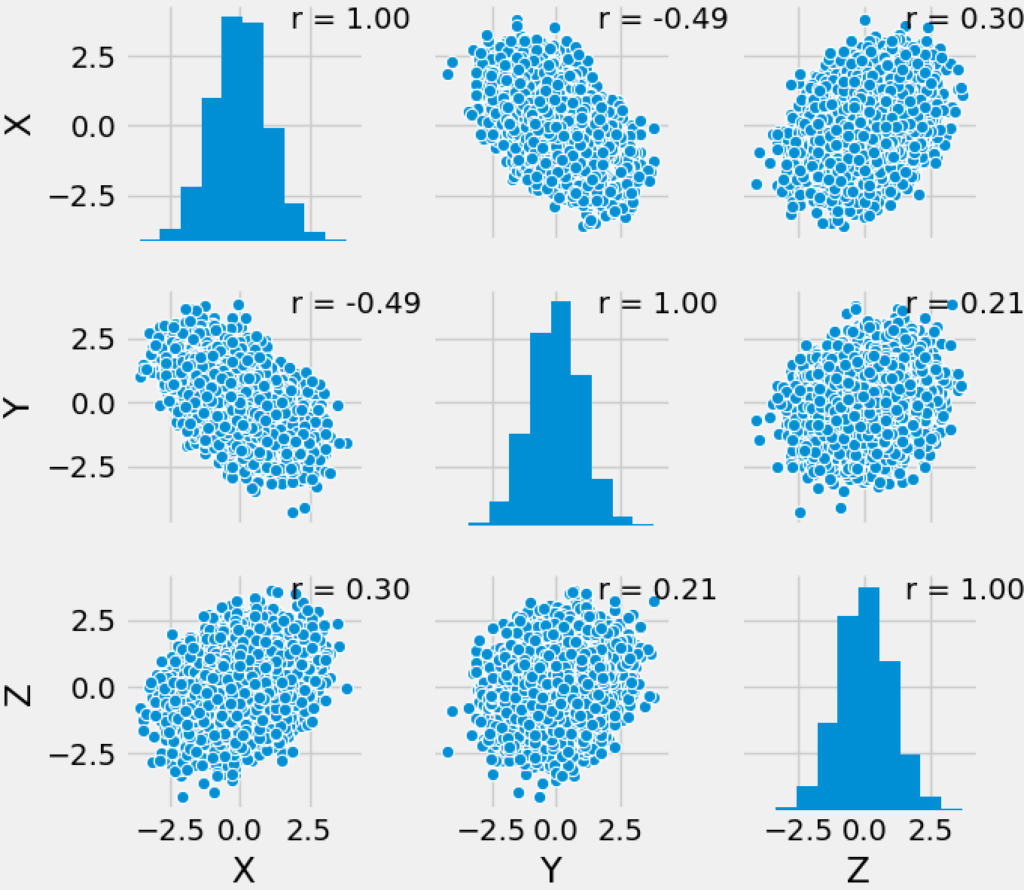
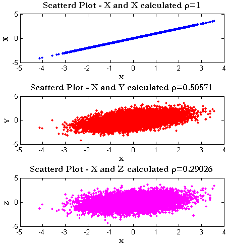
Matlab code
x=[  1  0.5 0.3; 0.5  1  0.3; 0.3 0.3  1 ;]; %Correlation matrix
U=chol(x); %Cholesky decomposition

R=randn(10000,3); %Random data in three columns each for X,Y and Z
Rc=R*U; %Correlated matrix Rc=[X Y Z]

%Verify Correlation-Coeffs of generated vectors
coeffMatrixXX=corrcoef(Rc(:,1),Rc(:,1));
coeffMatrixXY=corrcoef(Rc(:,1),Rc(:,2));
coeffMatrixXZ=corrcoef(Rc(:,1),Rc(:,3));

%Extract the required correlation coefficients
coeffXX=coeffMatrixXX(1,2) %Correlation Coeff for XX;
coeffXY=coeffMatrixXY(1,2) %Correlation Coeff for XY;
coeffXZ=coeffMatrixXZ(1,2) %Correlation Coeff for XZ;

%Scatterplots
subplot(3,1,1)
plot(Rc(:,1),Rc(:,1),'b.')
title(['Scatterd Plot - X and X calculated \rho=' num2str(coeffXX)])
xlabel('X')
ylabel('X')

subplot(3,1,2)
plot(Rc(:,1),Rc(:,2),'r.')
title(['Scatterd Plot - X and Y calculated \rho=' num2str(coeffXY)])
xlabel('X')
ylabel('Y')

subplot(3,1,3)
plot(Rc(:,1),Rc(:,3),'m.')
title(['Scatterd Plot - X and Z calculated \rho=' num2str(coeffXZ)])
xlabel('X')
ylabel('Z')
Scattered plots to verify the simulated data
Rate this article: [ratings]
Further reading
Topics in this chapter
[table “33” not found /]Books by the author
[table “23” not found /]