This post contains interactive python code which you can execute in the browser itself.
Central Limit Theorem – What is it ?
The central limit theorem (CLT) is a fundamental concept in statistics and probability theory that explains how the sum of independent and identically distributed random variables behaves. The theorem states that as the number of these variables increases, the distribution of their sum tends to become more like a normal distribution, even if the variables themselves are not normally distributed.
CLT states that the sum of independent and identically distributed (i.i.d) random variables (with finite mean and variance) approaches normal distribution as sample size \(N \rightarrow \infty\). In simpler terms, the theorem states that under certain general conditions, the sum of independent observations that follow same underlying distribution approximates to normal distribution. The approximation steadily improves as the number of observations increase. The underlying distribution of the independent observation can be anything – binomial, Poisson, exponential, Chi-Squared etc.
Why CLT ?
CLT is an important concept in statistics because it allows us to make inferences about a population based on a sample, even if we do not know the distribution of the population. It is used in many statistical techniques, such as hypothesis testing and confidence intervals.
Applications of CLT
Central limit theorem (CLT) is applied in a vast range of applications including (but not limited to) signal processing, channel modeling, random process, population statistics, engineering research, predicting the confidence intervals, hypothesis testing, etc. One such application in signal processing is – deriving the response of a cascaded series of low pass filters by applying the CLT. In the article titled ‘the central limit theorem and low-pass filters‘ the author has illustrated how the response of a cascaded series of low pass filters approaches Gaussian shape as the number of filters in the series increase [1].
In digital communication, the effect of noise on a communication channel is modeled as additive Gaussian white noise. This follows from the fact that the noise from many physical channels can be considered approximately Gaussian. For example, the random movement of electrons in the semiconductor devices gives rise to shot noise whose effect can be approximated to Gaussian distribution by applying central limit theorem.
Law of large numbers and CLT
there is a connection between the central limit theorem and the law of large numbers.
The law of large numbers is another important theorem in probability theory, which states that as the number of independent and identically distributed (iid) random variables increases, the average of those variables converges to the expected value of the distribution. In other words, as the sample size increases, the sample mean becomes more and more representative of the true population mean.
The central limit theorem, on the other hand, describes the distribution of the sum of iid random variables, and shows that as the sample size increases, the distribution of the sum approaches a normal distribution.
Both the law of large numbers and the CLT deal with the behavior of the sum or average of iid random variables as the sample size gets larger. The law of large numbers describes the behavior of the sample mean, while the CLT describes the behavior of the sum of the variables.
In essence, the law of large numbers is a precursor to the central limit theorem, as it establishes the fact that the sample mean becomes more and more representative of the true population mean as the sample size increases, and the central limit theorem shows that the distribution of the sum of iid random variables approaches a normal distribution as the sample size gets larger.
Demonstration using Python
For Matlab code, please refer the following book – Wireless communication systems in Matlab – by Mathuranathan Viswanathan
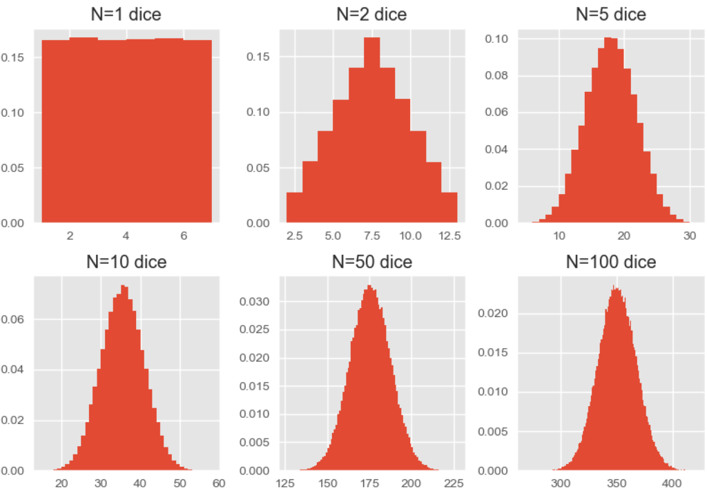
The following Python code illustrate how the theorem comes to play when the number of observations is increased for two separate experiments: rolling \(N\) unbiased dice and tossing \(N\) unbiased coins. The code generates \(N\) i.i.d discrete uniform random variables that generates uniform random numbers from the set \(\left\{1,k\right\}\). In the case of the dice rolling experiment, \(k\) is set to \(6\), thus simulating the random pick from the sample space \(S=\left\{1,2,3,4,5,6\right\}\) with equal probability. For the coin tossing experiment, \(k\) is set to \(2\), thus simulating the sample space of \(S=\left\{1,2\right\}\) representing head or tail events with equal probability. Rest of the code is self explanatory.
Python code
Run the following interactive code to see the results below
Simulation results
Reference images