Key focus: Colored noise sequence (a.k.a correlated Gaussian sequence), is a non-white random sequence, with non-constant power spectral density across frequencies.
Introduction
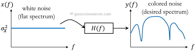
Speaking of Gaussian random sequences such as Gaussian noise, we generally think that the power spectral density (PSD) of such Gaussian sequences is flat.We should understand that the PSD of a Gausssian sequence need not be flat. This bring out the difference between white and colored random sequences, as captured in Figure 1.
A white noise sequence is defined as any random sequence whose PSD is constant across all frequencies. Gaussian white noise is a Gaussian random sequence, whose amplitude is gaussian distributed and its PSD is a constant. Viewed in another way, a constant PSD in frequency domain implies that the average auto-correlation function in time-domain is an impulse function (Dirac-delta function). That is, the amplitude of noise at any given time instant is correlated only with itself. Therefore, such sequences are also referred as uncorrelated random sequences. White Gaussian noise processes are completely characterized by its mean and variance.
[table “36” not found /]
A colored noise sequence is simply a non-white random sequence, whose PSD varies with frequency. For a colored noise, the amplitude of noise at any given time instant is correlated with the amplitude of noise occurring at other instants of time. Hence, colored noise sequences will have an auto-correlation function other than the impulse function. Such sequences are also referred as correlated random sequences. Colored
Gaussian noise processes are completely characterized by its mean and the shaped of power spectral density (or the shape of auto-correlation function).
In mobile channel model simulations, it is often required to generate correlated Gaussian random sequences with specified mean and power spectral density (like Jakes PSD or Gaussian PSD given in section 11.3.2 in the book). An uncorrelated Gaussian sequence can be transformed into a correlated sequence through filtering or linear transformation, that preserves the Gaussian distribution property of amplitudes, but alters only the correlation property (equivalently the power spectral density). We shall see two methods to generate colored Gaussian noise for given mean and PSD shape
• Spectral factorization method
• Auto-regressive (AR) model
Motivation
Let’s say we observe a real world signal $latex y[n]$ that has an arbitrary spectrum $latex y(f)$. We would like to describe the long sequence of $latex y[n]$ using very few parameters, as in applications like linear predictive coding (LPC). The modeling approach, described here, tries to answer the following two questions:
• Is it possible to model the first order (mean/variance) and second order (correlations, spectrum) statistics of the signal just by shaping a white noise spectrum using a transfer function ? (see Figure 1).
• Does this produce the same statistics (spectrum, correlations, mean and variance) for a white noise input ?
If the answer is yes to the above two questions, we can simply set the modeled parameters of the system and excite the system with white noise, to produce the desired real world signal. This reduces the amount to data we wish to transmit in a communication system application. This approach can be used to transform an uncorrelated white Gaussian noise sequence to a colored Gaussian noise sequence with desired spectral properties.
Linear time invariant (LTI) system model
In the given model, the random signal $latex y[n]$ is observed. Given the observed signal $latex y[n]$, the goal here is to find a model that best describes the spectral properties of $latex y[n]$ under the following assumptions
• The sequence $latex y[n]$ is WSS (wide sense stationary) and ergodic.
• The input sequence $latex x[n]$ to the LTI system is white noise, whose amplitudes follow Gaussian distribution with zero-mean and variance $latex \sigma_x^2$ with flat the power spectral density.
• The LTI system is BIBO (bounded input bounded output) stable.
Read the continuation of this post : Spectral factorization method
Rate this article: [ratings]
Reference
Books by the author
[table “23” not found /]