Partial response schemes: impulse & frequency response

Impulse response and frequency response of PR signaling schemes

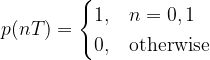
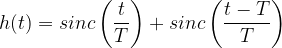
Consider a minimum bandwidth system in which the filter is represented as a cascaded combination of a partial response filter and a minimum bandwidth filter . Since is a brick-wall filter, the frequency response of the whole system is equivalent to frequency response of the FIR filter , whose transfer function, for various partial response schemes, was listed in Table 1 in the previous post (shown below).

Table 1: Partial response signaling schemes
Table 1: Partial response signaling schemes

The hand-crafted Matlab function (given in the book) generates the overall partial response signal for the given transfer function . The function records the impulse response of the filter by sending an impulse through it. These samples are computed at each symbol sampling instants. In order to visualize the pulse shaping functions and to compute the frequency response, the impulse response of are oversampled by a factor . This converts the samples from symbol rate domain to sampling rate domain. The oversampled impulse response of filter is convolved with a sinc filter that satisfies the Nyquist first criterion. This results in the overall response of the equivalent filter (refer Figure 2 in the previous post).

This article is part of the book Wireless Communication Systems in Matlab, ISBN: 978-1720114352 available in ebook (PDF) format (click here) and Paperback (hardcopy) format (click here).

The Matlab code to simulate both the impulse response and the frequency response of various PR signaling schemes, is given next (refer book for the Matlab code). The simulated results are plotted in the following Figure.

Figure: Impulse response and frequency response of various Partial response (PR) signaling schemes

Rate this post: Note: There is a rating embedded within this post, please visit this post to rate it.

Books by the author


Wireless Communication Systems in Matlab
Second Edition(PDF)

Note: There is a rating embedded within this post, please visit this post to rate it.
Checkout Added to cart

Digital Modulations using Python
(PDF ebook)

Note: There is a rating embedded within this post, please visit this post to rate it.
Checkout Added to cart

Digital Modulations using Matlab
(PDF ebook)

Note: There is a rating embedded within this post, please visit this post to rate it.
Checkout Added to cart
Hand-picked Best books on Communication Engineering
Best books on Signal Processing

Topics in this chapter

Pulse Shaping, Matched Filtering and Partial Response Signaling
● Introduction
● Nyquist Criterion for zero ISI
● Discrete-time model for a system with pulse shaping and matched filtering
 □ Rectangular pulse shaping
 □ Sinc pulse shaping
 □ Raised-cosine pulse shaping
 □ Square-root raised-cosine pulse shaping
● Eye Diagram
● Implementing a Matched Filter system with SRRC filtering
 □ Plotting the eye diagram
 □ Performance simulation
● Partial Response Signaling Models
 □ Impulse response and frequency response of PR signaling schemes
● Precoding
 □ Implementing a modulo-M precoder
 □ Simulation and results

Partial response (PR) signaling Model

Consider the generic baseband communication system model and its equivalent representation, shown in Figure 1, where the various blocks in the system are represented as filters. To have no ISI at the symbol sampling instants, the equivalent filter should satisfy Nyquist’s first criterion.

Figure 1: A generic communication system model and its equivalent representation

If the system is ideal and noiseless, it can be characterized by samples of the desired impulse response . Let’s represent all the non-zero sample values of the desired impulse response, taken at symbol sampling spacing , as , for .

This article is part of the book
Wireless Communication Systems in Matlab (second edition), ISBN: 979-8648350779 available in ebook (PDF) format and Paperback (hardcopy) format.

The partial response signaling model, illustrated in Figure 2, is expressed as a cascaded combination of a tapped delay line filter with tap coefficients set to and a filter with frequency response . The filter forces the desired sample values. On the other hand, the filter bandlimits the system response and at the same time it preserves the sample values from the filter . The choice of filter coefficients for the filter and the different choices for for satisfying Nyquist first criterion, result in different impulse response , but renders identical sample values in Figure 2 [1].

Figure 2: A generic partial response (PR) signaling model

To have a system with minimum possible bandwidth, the filter is chosen as

The inverse Fourier transform of results in a sinc pulse. The corresponding overall impulse response of the system is given by

If the bandwidth can be relaxed, other ISI free pulse-shapers like raised cosine can be considered for the filter.

Given the nature of real world channels, it is not always desirable to satisfy Nyquist’s first criterion. For example, the channel in magnetic recording, exhibits spectral null at certain frequencies and therefore it defines the channel’s upper frequency limit. In such cases, it is very difficult to satisfy Nyquist first criterion. An alternative viable solution is to allow a controlled amount of ISI between the adjacent samples at the output of the equivalent filter shown in Figure 2. This deliberate injection of controlled amount of ISI is called partial response (PR) signaling or correlative coding.

Partial Response Signaling Schemes

Several classes of PR signaling schemes and their corresponding transfer functions represented as (where is the delay operator) are shown in Table 1. The unit delay is equal to a delay of 1 symbol duration () in a continuous time system.

Rate this article: Note: There is a rating embedded within this post, please visit this post to rate it.

References

[1] Peter Kabal and Subbarayan Pasupathy, Partial-response signaling, IEEE Transactions on Communications, Vol. 23, No. 9, pp. 921-934, September 1975.↗

Topics in this chapter

Pulse Shaping, Matched Filtering and Partial Response Signaling
● Introduction
● Nyquist Criterion for zero ISI
● Discrete-time model for a system with pulse shaping and matched filtering
 □ Rectangular pulse shaping
 □ Sinc pulse shaping
 □ Raised-cosine pulse shaping
 □ Square-root raised-cosine pulse shaping
● Eye Diagram
● Implementing a Matched Filter system with SRRC filtering
 □ Plotting the eye diagram
 □ Performance simulation
● Partial Response Signaling Models
 □ Impulse response and frequency response of PR signaling schemes
● Precoding
 □ Implementing a modulo-M precoder
 □ Simulation and results

Books by the author


Wireless Communication Systems in Matlab
Second Edition(PDF)

Note: There is a rating embedded within this post, please visit this post to rate it.
Checkout Added to cart

Digital Modulations using Python
(PDF ebook)

Note: There is a rating embedded within this post, please visit this post to rate it.
Checkout Added to cart

Digital Modulations using Matlab
(PDF ebook)

Note: There is a rating embedded within this post, please visit this post to rate it.
Checkout Added to cart
Hand-picked Best books on Communication Engineering
Best books on Signal Processing

Correlative Coding – Modified Duobinary Signaling

Modified Duobinary Signaling is an extension of duobinary signaling. It has the advantage of zero PSD at low frequencies (especially at DC ) that is suitable for channels with poor DC response. It correlates two symbols that are 2T time instants apart, whereas in duobinary signaling, symbols that are 1T apart are correlated.

The general condition to achieve zero ISI is given by

As discussed in a previous article, in correlative coding , the requirement of zero ISI condition is relaxed as a controlled amount of ISI is introduced in the transmitted signal and is counteracted in the receiver side

In the case of modified duobinary signaling, the above equation is modified as

which states that the ISI is limited to two alternate samples. Here a controlled or “deterministic” amount of ISI is introduced and hence its effect can be removed upon signal detection at the receiver.

Modified Duobinary Signaling:

The following figure shows the modified duobinary signaling scheme (click to enlarge).

Modified DuoBinary Signaling

Encoding Process:

1) an = binary input bit; an ∈ {0,1}.
2) bn = NRZ polar output of Level converter in the precoder and is given by,

where ak is the precoded output (before level converter).

3) yn can be represented as

Note that the samples bn are uncorrelated ( i.e either +d for “1” or -d for “0” input). On the other-hand,the samples yn are correlated ( i.e. there are three possible values +2d,0,-2d depending on ak and ak-2). Meaning that the modified duobinary encoding correlates present sample ak and the previous input sample ak-2.

4) From the diagram,impulse response of the modified duobinary encoder is computed as

Decoding Process:

5) The receiver consists of a modified duobinary decoder and a postcoder (inverse of precoder). The decoder implements the following equation (which can be deduced from the equation given under step 3 (see above))

This equation indicates that the decoding process is prone to error propagation as the estimate of present sample relies on the estimate of previous sample. This error propagation is avoided by using a precoder before modified-duobinary encoder at the transmitter and a postcoder after the modified-duobinary decoder. The precoder ties the present sample and the sample that precedes the previous sample ( correlates these two samples) and the postcoder does the reverse process.

6) The entire process of modified-duobinary decoding and the postcoding can be combined together as one algorithm. The following decision rule is used for detecting the original modified-duobinary signal samples {an} from {yn}

Matlab code:

Check this book for full Matlab code.
Wireless Communication Systems in Matlab – by Mathuranathan Viswanathan

Simulation Results:

To know more on the simulation and results – visit this page – “Partial response signalling schemes – impulse and frequency responses”

Impulse response and frequency response of various Partial response (PR) signaling schemes

Rate this post: Note: There is a rating embedded within this post, please visit this post to rate it.

See also :

[1] Correlative Coding – Duobinary Signaling
[2] Introduction to Inter Symbol Interference

Recommended Books

Correlative coding – Duobinary Signaling

The condition for zero ISI (Inter Symbol Interference) is

which states that when sampling a particular symbol (at time instant nT=0), the effect of all other symbols on the current sampled symbol is zero.

As discussed in the previous article, one of the practical ways to mitigate ISI is to use partial response signaling technique ( otherwise called as “correlative coding”). In partial response signaling, the requirement of zero ISI condition is relaxed as a controlled amount of ISI is introduced in the transmitted signal and is counteracted in the receiver side.

By relaxing the zero ISI condition, the above equation can be modified as,

which states that the ISI is limited to two adjacent samples. Here we introduce a controlled or “deterministic” amount of ISI and hence its effect can be removed upon signal detection at the receiver.

Duobinary Signaling:

The following figure shows the duobinary signaling scheme.

Figure 1: DuoBinary signaling scheme

Encoding Process:

1) an = binary input bit; an ∈ {0,1}.
2) bn = NRZ polar output of Level converter in the precoder and is given by,

3) yn can be represented as

Note that the samples bn are uncorrelated ( i.e either +d for “1” or -d for “0” input). On the other-hand, the samples yn are correlated ( i.e. there are three possible values +2d,0,-2d depending on an and an-1). Meaning that the duobinary encoding correlates present sample an and the previous input sample an-1.

4) From the diagram,impulse response of the duobinary encoder is computed as

Decoding Process:

5) The receiver consists of a duobinary decoder and a postcoder (inverse of precoder).The duobinary decoder implements the following equation (which can be deduced from the equation given under step 3 (see above))

This equation indicates that the decoding process is prone to error propagation as the estimate of present sample relies on the estimate of previous sample. This error propagation is avoided by using a precoder before duobinary encoder at the transmitter and a postcoder after the duobinary decoder. The precoder ties the present sample and previous sample ( correlates these two samples) and the postcoder does the reverse process.

6) The entire process of duobinary decoding and the postcoding can be combined together as one algorithm. The following decision rule is used for detecting the original duobinary signal samples {an} from {yn}

Matlab Code:

Check this book for full Matlab code and simulation results.
Wireless Communication Systems in Matlab – by Mathuranathan Viswanathan

Simulation and results

To know more on the simulation and results – visit this page – “Partial response signalling schemes – impulse and frequency responses”

Impulse response and frequency response of various Partial response (PR) signaling schemes

Rate this article: Note: There is a rating embedded within this post, please visit this post to rate it.

See also :

[1] Correlative Coding – Modified Duobinary Signaling
[2] Derivation of expression for a Gaussian Filter with 3 dB bandwidth
[3] Nyquist and Shannon Theorem
[4] Correlative coding – Duobinary Signaling
[5] Square Root Raised Cosine Filter (Matched/split filter implementation)
[6] Introduction to Inter Symbol Interference

External Resources:

[1] The care and feeding of digital, pulse-shaping filters – By Ken Gentile↗
[2] Inter Symbol Interference and Root Raised Cosine Filtering – Complex2real↗