
Pulse-shaping Lab path:
Nyquist zero-ISI → Raised cosine → Matched filter + SRRC → Eye diagrams
Tool: RRC filter & bandwidth calculator
In digital communications, an eye diagram (or eye pattern) is one of the most intuitive and powerful diagnostic tools for evaluating signal quality. Formed by overlapping consecutive symbol traces of a modulated signal over a fixed time window, the eye diagram instantly reveals the combined effects of Inter-Symbol Interference (ISI), phase jitter, dynamic range limitations, and noise.
While real-time digital sampling oscilloscopes (DSOs) construct eye diagrams directly from physical voltage measurements, digital communication system simulations—whether in MATLAB, Python, or C++—operate on sampled discrete-time vectors in memory.
This guide explains the step-by-step mathematical mechanics of constructing an eye diagram from computer memory, avoiding common sampling traps, and implementing vectorized plotting in both MATLAB and Python.
1. Key Parameters Required for Eye Diagram Generation
To construct a mathematically accurate eye diagram from a continuous-time simulation vector $r(t)$ or discrete vector $r[n]$, you must know three fundamental system parameters:
- Symbol Rate ($R_s = 1 / T_s$): The number of symbols transmitted per second (Baud rate), where $T_s$ is the symbol duration.
- Sampling Frequency ($F_s = 1 / T_{sample}$): The rate at which the continuous waveform was digitized.
- Oversampling Factor ($L = N_{spb}$): The number of samples per symbol (or Samples Per Bit for binary signaling):
$$L = \frac{F_s}{R_s} = \frac{T_s}{T_{sample}}$$
Rule of Thumb: To generate a smooth visual eye diagram without artificial linear interpolations, the signal must be oversampled by at least $L \ge 8$ or $L \ge 16$ samples per symbol. If your simulation operates at baseband with $L = 2$ (e.g., for matched filtering), upsample the signal using polyphase FIR interpolation (
resampleorscipy.signal.resample) before plotting.
2. Step-by-Step Matrix Reshaping Mechanics
Instead of using slow for loops to slice a vector into individual trace segments, we leverage matrix reshaping to stack consecutive symbol intervals into array columns.
Assume we want to display an eye diagram over a window of $K$ symbol intervals (typically $K = 2$ or $K = 3$ symbols wide):
- Define Trace Length: Each trace sweep contains $M = K \times L$ samples.
- Segment the Vector: Truncate the discrete signal vector $x[n]$ so its total length is an integer multiple of the trace length $M$.
- Matrix Reshaping: Reshape the $1 \times (N \cdot M)$ vector into an $M \times N$ matrix, where each column represents one visual trace across $K$ symbol periods:
$$\mathbf{X} = \begin{bmatrix} x[0] & x[M] & x[2M] & \dots \\ x[1] & x[M+1] & x[2M+1] & \dots \\ \vdots & \vdots & \vdots & \ddots \\ x[M-1] & x[2M-1] & x[3M-1] & \dots \end{bmatrix}$$ - Time Axis Mapping: Create a time vector $t_{axis} = [0, 1, \dots, M-1] \times T_{sample}$ mapped to normalized symbol times (e.g., $t / T_s \in [0, K]$).
3. MATLAB Implementation
The standard MATLAB eyediagram function from the Communications Toolbox is convenient, but constructing your own vectorized engine offers total flexibility for custom UI overlays, export quality, and zero-toolbox dependencies.
Matlab
% Construction of Eye Diagram from Memory Vector in MATLAB
clear; clc; close all;

%% 1. System Parameters
M_ary = 4;                 % 4-PAM Modulation
numSymbols = 2000;         % Number of transmitted symbols
L = 16;                    % Oversampling Factor (Samples/Symbol)
K = 2;                     % Eye Diagram Display Window (in Symbol Durations)
rolloff = 0.35;            % Pulse Shaping Roll-off factor

%% 2. Generate Bandlimited Waveform (with ISI and Noise)
data = randi([0 M_ary-1], numSymbols, 1);
symbols = pammod(data, M_ary, 0, 'gray');

% Upsample and Apply Root-Raised Cosine (RRC) Pulse Shaping Filter
symbolsUp = upsample(symbols, L);
rrcFilter = rcosdesign(rolloff, 6, L, 'sqrt');
txWaveform = conv(symbolsUp, rrcFilter, 'same');

% Add Channel AWGN Noise
rxWaveform = awgn(txWaveform, 22, 'measured');

%% 3. Matrix Reshaping Engine
samplesPerTrace = K * L;
numTraces = floor(length(rxWaveform) / samplesPerTrace);

% Truncate and reshape vector into [samplesPerTrace x numTraces]
signalMatrix = reshape(rxWaveform(1:numTraces * samplesPerTrace), samplesPerTrace, numTraces);

% Normalize Time Axis to Symbol Period (t / Ts)
t_axis = (0:samplesPerTrace-1) / L;

%% 4. Vectorized Plotting
figure('Color', [1 1 1]);
plot(t_axis, signalMatrix, 'b-', 'LineWidth', 0.5);
grid on;
title(sprintf('Eye Diagram (%d-PAM, Roll-off = %.2f)', M_ary, rolloff));
xlabel('Time (t / T_s)');
ylabel('Amplitude');
xlim([0 K]);
4. Python Implementation (NumPy & Matplotlib)
Here is the equivalent implementation in Python using NumPy matrix manipulation and Matplotlib vectorization:
Python
import numpy as np
import matplotlib.pyplot as plt
from scipy.signal import firwin, lfilter

# 1. System Setup
num_symbols = 2500
L = 16          # Oversampling factor (samples/symbol)
K = 2           # 2-symbol window
rolloff = 0.35

# 2. Generate BPSK Symbol Sequence
symbols = 2 * np.random.randint(0, 2, num_symbols) - 1

# Upsample
symbols_up = np.zeros(num_symbols * L)
symbols_up[::L] = symbols

# Simple RC-like Pulse Shaping Filter
num_taps = 6 * L + 1
t = np.arange(-3 * L, 3 * L + 1) / L
h_rc = np.sinc(t) * np.cos(np.pi * rolloff * t) / (1 - (2 * rolloff * t)**2 + 1e-12)
rx_waveform = np.convolve(symbols_up, h_rc, mode='same')

# Add Gaussian Noise
noise = np.random.normal(0, 0.15, len(rx_waveform))
rx_waveform += noise

# 3. Reshape Signal Vector
samples_per_trace = K * L
num_traces = len(rx_waveform) // samples_per_trace
eye_matrix = rx_waveform[:num_traces * samples_per_trace].reshape((num_traces, samples_per_trace)).T

# 4. Plot Eye Diagram
t_axis = np.arange(samples_per_trace) / L

plt.figure(figsize=(8, 5))
plt.plot(t_axis, eye_matrix, color='#1e3a8a', alpha=0.15, linewidth=0.8)
plt.grid(True, linestyle='--', alpha=0.6)
plt.title(f'Eye Diagram (BPSK, {L} Samples/Symbol)', fontsize=12, fontweight='bold')
plt.xlabel('Time (t / $T_s$)')
plt.ylabel('Amplitude')
plt.xlim(0, K)
plt.tight_layout()
plt.show()
5. How to Read Key Metrics from an Eye Diagram
An eye diagram acts as a visual summary of system performance:
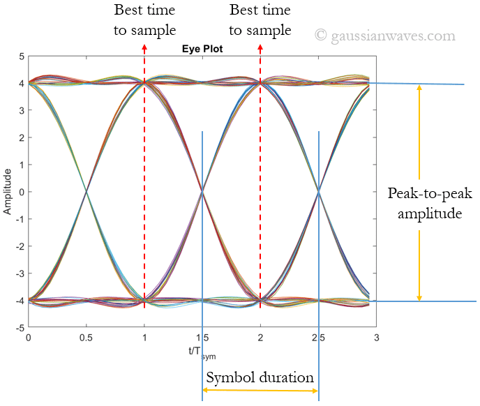
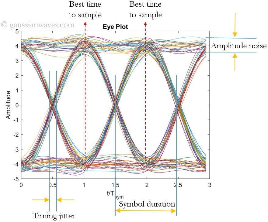
- Eye Opening (Height): Measured vertically at the optimum sampling instant ($t = T_s/2$). A wide vertical opening indicates high Noise Margin and low ISI.
- Eye Width: Measured horizontally at the zero-crossing line. Indicates signal tolerance to timing jitter and clock phase errors.
- Jitter (Timing Noise): The horizontal thickness of the edge transition crossings. Broader crossings indicate high phase noise or residual channel dispersion.
- Sensitivity / Slope: The slope of the opening edges dictates how sensitive the system is to sample timing offsets. Steeper slopes mean small timing errors cause large voltage degradation.
6. Common Pitfalls & Practical Tips
- Filter Delay Alignment: Group delay introduced by pulse shaping filters (RRC/RC) shifts the optimum sampling point. Make sure to prune or align the filter delay before reshaping, or the eye opening will be offset from the center of the plot.
- Carrier Frequency Offset (CFO): If residual frequency offset remains in a complex baseband signal ($I + jQ$), the constellation rotates over time, causing the eye diagram to close completely. Always plot eye diagrams on either the In-phase ($I$) or Quadrature ($Q$) rail after carrier recovery.
- Color Density (Heatmap Eye Diagrams): For large vectors ($>100,000$ symbols), standard line plots become slow and muddy. Instead of plotting individual line paths, compute a 2D histogram of time vs. amplitude (
matplotlib.pyplot.hist2d) to create an oscilloscope-style persistence density eye map.
Further reading
[1] Tektronix application note: Anatomy of an eye diagram.↗
[2] Anritsu application note: Understanding eye pattern measurements.↗