Let’s learn the equations and the filter model for simulating square root raised cosine (SRRC) pulse shaping. Before proceeding, I urge you to read about basics of pulse shaping in this article.
Raised-cosine pulse shaping filter is generally employed at the transmitter. Let $latex X_{rc} (f)$ be the raised cosine filter’s frequency response. Assume that the channel’s amplitude response is flat, i.e, $latex H_c(f)=1$ and the channel noise is white. Then, the combined response of the transmit filter $latex P(f)$ and receiver filter $latex G(f)$ in frequency domain is given as

If the receive filter is matched with the transmit filter, we have

Thus, the transmit and the receive filter take the form

with $latex G(f) = P^{\ast}(f)$, where $latex T_0$ is a nominal delay that is required to ensure the practical realizability of the filters. In time domain, a matched filter at the receiver is the mirrored copy of the impulse response of the transmit pulse shaping filter and is delayed by some time $latex T_0$. Thus the task of raised cosine filtering is equally split between the transmit and receive filters. This gives rise to square-root raised-cosine (SRRC) filters at the transmitter and receiver, whose equivalent impulse response is described as follows.

[table “36” not found /]
The roll-of factor for the SRRC is denoted as $latex \beta$ to distinguish it from that of the RC filter. A simple evaluation of the equation (4) produces singularities (undefined points) at $latex p(t=0)$ and $latex p(t=\pm \frac{T_{sym}}{4 \beta})$. The value of the square root raised cosine pulse at these singularities can be obtained by applying L’Hostipital’s rule [1] and the values are

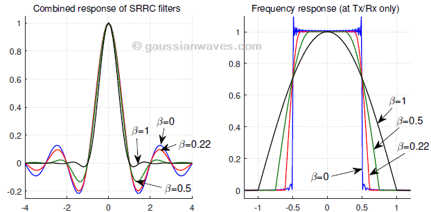
A function for generating SRRC pulse shape is given next. It is followed by a test code that plots the combined impulse response of transmit-receive SRRC filter combination and also plots the frequency domain view of a single SRRC pulse as shown in Figure 1
The combined impulse response matters, as we can identify that the combined response hits zero at symbol sampling instants. This indicates that the job of ISI cancellation is split between transmitter and receiver filters. Note that the combined impulse response of two SRRC filters is same as the impulse response of the RC filter.
Program 1: srrcFunction.m: Function for generating square-root raised-cosine pulse (click here)
Program 2: test_SRRCPulse.m: Square-root raised-cosine pulse characteristics
Tsym=1; %Symbol duration in seconds
L=10; % oversampling rate, each symbol contains L samples
Nsym = 80; %filter span in symbol durations
betas=[0 0.22 0.5 1];%root raised-cosine roll-off factors
Fs=L/Tsym;%sampling frequency
lineColors=['b','r','g','k','c']; i=1;legendString=cell(1,4);
for beta=betas %loop for various alpha values
	[srrcPulseAtTx,t]=srrcFunction(beta,L,Nsym); %SRRC Filter at Tx
	srrcPulseAtRx = srrcPulseAtTx;%Using the same filter at Rx
	%Combined response matters as it hits 0 at desired sampling instants
	combinedResponse = conv(srrcPulseAtTx,srrcPulseAtRx,'same');

	subplot(1,2,1); t=Tsym*t; %translate time base & normalize reponse
	plot(t,combinedResponse/max(combinedResponse),lineColors(i));
	hold on;

	%See Chapter 1 for the function 'freqDomainView'
	[vals,F]=freqDomainView(srrcPulseAtTx,Fs,'double');
	subplot(1,2,2);
	plot(F,abs(vals)/abs(vals(length(vals)/2+1)),lineColors(i));
	hold on;legendString{i}=strcat('\beta =',num2str(beta) );i=i+1;
end
subplot(1,2,1);
title('Combined response of SRRC filters'); legend(legendString);
subplot(1,2,2);
title('Frequency response (at Tx/Rx only)');legend(legendString);
References
- [1] Michael Joost, Theory of root-raised cosine filter, Research and Development, 47829 Krefeld, Germany, EU, Dec 2010. https://www.michael-joost.de/rrcfilter.pdf↗
Rate this article: [ratings]
Topics in this chapter
[table “27” not found /]Books by the author
[table “23” not found /]