The Nyquist-Shannon Sampling Theorem

Interactive lab: open the Nyquist sampling & aliasing demo for baseband Fs regimes, then the bandpass sampling demo when the signal lives in a band away from DC.

Think of the sampling theorem as the bridge between the continuous analog world (sound waves, radio signals, voltages) and the discrete digital world ($1\text{s}$ and $0\text{s}$ in computers).

The Wagon-Wheel Effect

Have you ever watched a movie where a car accelerates, and suddenly the spokes on the wheels look like they are spinning backwards or standing completely still?

That is Aliasing!

• A movie camera takes snapshots (samples) at 24 frames per second ($24\text{ Hz}$).
• When the wheel rotates faster than half the camera’s frame rate ($12\text{ rotations/second}$), the camera fails to capture the true forward motion and creates a false, lower-frequency optical illusion.

In digital audio or communications, if you sample continuous signals too slowly, high frequencies disguise themselves as low frequencies, permanently ruining the recording.

The Core Mathematical Rule

If a continuous signal $x(t)$ contains no frequency components higher than $F_m\text{ Hertz}$ (its bandwidth), you can perfectly reconstruct $x(t)$ from its discrete samples $x[n] = x(n T_s)$ if and only if the sampling rate $F_s$ satisfies:

$$F_s \ge 2 F_m$$

Where:

• $F_s = \frac{1}{T_s}$ is the Sampling Frequency (samples per second).
• $T_s$ is the Sampling Interval (time between consecutive snapshots).
• $F_m$ is the Maximum Frequency present in the signal.

Key Terminology:

1. Nyquist Rate ($2 F_m$): The minimum speed at which you must sample a signal without losing information.
2. Nyquist Frequency ($F_s / 2$): The maximum signal frequency that a system sampling at rate $F_s$ can safely process. This is also called the folding frequency.

What Happens in the Frequency Domain?

To understand why $F_s \ge 2 F_m$ works, look at what sampling actually does in the frequency spectrum:

1. Continuous Spectrum: A continuous signal has a single spectrum bounded between $-F_m$ and $+F_m$.
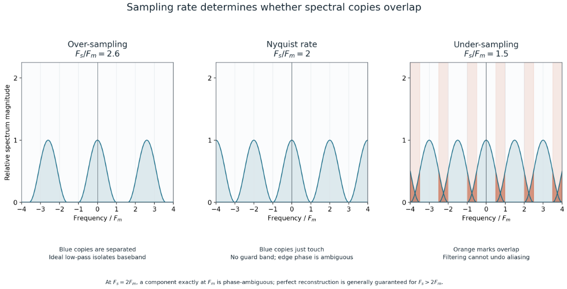
2. Sampling Effect: Periodically taking samples in the time domain creates infinite repeating copies (spectral replicas) of the signal’s spectrum in the frequency domain, centered at multiples of the sampling frequency ($\dots, -2F_s, -F_s, 0, +F_s, +2F_s, \dots$).

• Case 1: Over-sampling ($F_s > 2 F_m$)The spectral copies are separated by a safety distance called a guard band. A low-pass filter can easily isolate the original spectrum centered at $0\text{ Hz}$.
• Case 2: Under-sampling ($F_s < 2 F_m$) — Aliasing Occurs!The spectral copies overlap each other. High-frequency information spills into the baseband spectrum. Once overlapping occurs, no filter in the world can separate the original signal from the distortion.

Signal Reconstruction (Sinc Interpolation)

To convert discrete samples $x[n]$ back into a continuous signal $x(t)$, we pass the samples through an ideal low-pass filter with cutoff frequency $F_c = F_s / 2$.

In the time domain, this is equivalent to placing a Sinc function at every sample point:

$$x(t) = \sum_{n=-\infty}^{\infty} x(n T_s) \cdot \operatorname{sinc}\left( \frac{t – n T_s}{T_s} \right)$$

Where $\operatorname{sinc}(u) = \frac{\sin(\pi u)}{\pi u}$.

Each sinc curve reaches its peak value of $1.0$ at exact sample instant $t = n T_s$ and passes smoothly through zero at all other sample locations. Summing these weighted sinc waves fills in the gaps between sample points smoothly and perfectly.

Python Simulation: Nyquist Rate vs. Aliasing

Let’s write a Python script using numpy to demonstrate baseband sampling:

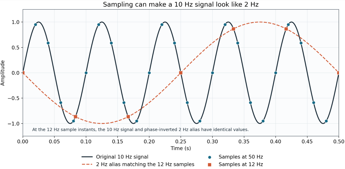
1. We create a continuous $10\text{ Hz}$ sine wave ($F_m = 10\text{ Hz}$). The true Nyquist rate is $2 \times 10 = 20\text{ Hz}$.
2. Proper Sampling ($F_s = 50\text{ Hz} > 20\text{ Hz}$): The signal is captured cleanly.
3. Under-Sampling ($F_s = 12\text{ Hz} < 20\text{ Hz}$): Aliasing occurs! The $10\text{ Hz}$ signal disguises itself as a false $\vert{}10 – 12\vert{} = 2\text{ Hz}$ sine wave.

import numpy as np

# --- 1. Continuous World Simulation ---
f_signal = 10.0          # Maximum signal frequency Fm = 10 Hz
t_duration = 1.0         # 1 second duration
f_analog = 2000.0        # High sample rate to emulate "continuous" analog wave
t_analog = np.arange(0, t_duration, 1.0 / f_analog)
x_analog = np.sin(2 * np.pi * f_signal * t_analog)

nyquist_rate = 2 * f_signal
print(f"Signal Frequency (Fm): {f_signal} Hz")
print(f"Theoretical Nyquist Rate (2*Fm): {nyquist_rate} Hz\n")

# --- 2. Case A: Proper Sampling (Fs = 50 Hz > 20 Hz) ---
Fs_proper = 50.0
t_proper = np.arange(0, t_duration, 1.0 / Fs_proper)
x_proper = np.sin(2 * np.pi * f_signal * t_proper)

# Measure dominant frequency in proper sampled signal using FFT
fft_proper = np.abs(np.fft.rfft(x_proper))
freqs_proper = np.fft.rfftfreq(len(x_proper), 1.0 / Fs_proper)
detected_freq_proper = freqs_proper[np.argmax(fft_proper)]

print("=== Case A: Proper Sampling (Fs = 50 Hz) ===")
print(f"Sampling Rate Fs: {Fs_proper} Hz (Fs > 2*Fm)")
print(f"Detected Baseband Frequency in Spectrum: {detected_freq_proper:.1f} Hz")
print("Status: Success! No Aliasing.\n")

# --- 3. Case B: Under-Sampling (Fs = 12 Hz < 20 Hz) ---
Fs_under = 12.0
t_under = np.arange(0, t_duration, 1.0 / Fs_under)
x_under = np.sin(2 * np.pi * f_signal * t_under)

# Measure dominant frequency in under-sampled signal using FFT
fft_under = np.abs(np.fft.rfft(x_under))
freqs_under = np.fft.rfftfreq(len(x_under), 1.0 / Fs_under)
detected_freq_under = freqs_under[np.argmax(fft_under)]

# Theoretical alias frequency formula: |f - k*Fs|
theoretical_alias = abs(f_signal - Fs_under)

print("=== Case B: Under-Sampling (Fs = 12 Hz) ===")
print(f"Sampling Rate Fs: {Fs_under} Hz (Fs < 2*Fm)")
print(f"Theoretical Aliased Frequency |10 - 12|: {theoretical_alias:.1f} Hz")
print(f"Detected Baseband Frequency in Spectrum: {detected_freq_under:.1f} Hz")
print("Status: ALIASING ERROR! 10 Hz signal appears as a 2 Hz ghost signal.")

Output

Signal Frequency (Fm): 10.0 Hz
Theoretical Nyquist Rate (2*Fm): 20.0 Hz

=== Case A: Proper Sampling (Fs = 50 Hz) ===
Sampling Rate Fs: 50.0 Hz (Fs > 2*Fm)
Detected Baseband Frequency in Spectrum: 10.0 Hz
Status: Success! No Aliasing.

=== Case B: Under-Sampling (Fs = 12 Hz) ===
Sampling Rate Fs: 12.0 Hz (Fs < 2*Fm)
Theoretical Aliased Frequency |10 - 12|: 2.0 Hz
Detected Baseband Frequency in Spectrum: 2.0 Hz
Status: ALIASING ERROR! 10 Hz signal appears as a 2 Hz ghost signal.

Summary Comparison

Sampling Scenario	Sampling Rate Condition	Spectral Relationship	Reconstruction Result
Over-sampling	$F_s > 2 F_m$	Spectral copies separated by guard bands	Perfect reconstruction possible
Nyquist Sampling	$F_s = 2 F_m$	Spectral copies touch edge-to-edge	Critical condition (requires exact phase alignment)
Under-sampling	$F_s < 2 F_m$	Spectral copies overlap (Aliasing)	Irreversible distortion (High frequencies impersonate low frequencies)

FAQ

Is the Nyquist rate a strict greater-than or greater-or-equal condition? Ideal sinc reconstruction of a signal bandlimited to $latex B$ requires $latex f_s>2B$. Equality is a mathematical boundary case; real ADCs add margin and rely on anti-alias filters that are not brick walls, so engineers treat $latex 2B$ as a lower bound to stay above.

Can passband signals be sampled slower than twice the highest frequency? Yes — intentional bandpass undersampling can alias a band down into baseband without overlap if the zone and bandwidth are chosen carefully. That does not violate Nyquist; it applies the theorem to the information bandwidth, not to the carrier frequency.

How does sampling rate show up in FFT bin spacing? Bin spacing is $latex f_s/N$. Raising $latex f_s$ stretches the Nyquist range but, for fixed $latex N$, makes each bin wider in hertz. Plan both with the FFT resolution calculator.

Reference:

[1] Claude E. Shannon, “Communication in the presence of noise” ,Proceedings of the IRE, Vol 37, no.1,pp.10-21,Jan 1949

Similar articles

• Analog vs discrete signals
• DFT bins & fftshift
• FFT calculator