Hata Okumura model for outdoor propagation

Outdoor propagation models involve estimation of propagation loss over irregular terrains such as mountainous regions, simple curved earth profile, etc., with obstacles like trees and buildings. All such models predict the received signal strength at a particular distance or on a small sector. These models vary in approach, accuracy and complexity. Hata Okumura model is one such model.

In 1986, Yoshihisa Okumura traveled around Tokyo city and made measurements for the signal attenuation from base station to mobile station. He came up with a set of curves which gave the median attenuation relative to free space path loss. Okumura came up with three set of data for three scenarios: open area, urban area and sub-urban area. Since this was one of the very first model developed for cellular propagation environment, there exist other difficulties and concerns related to the applicability of the model. Okumura model can be adopted for computer simulations by digitizing those curves provided by Okumura and using them in the form of look-up-tables [1]. Since it is based on empirical studies, the validity of parameters is limited in range. The parameter values outside the range can be obtained by extrapolating the curves. There are also concerns related to the calculation of effective antenna height. Thus every RF modeling tool incorporates its own interpretations and adjustments when it comes to implementing Okumura model.

Hata, in 1980, came up with closed form expressions based on curve fitting of Okumura models. It is the most referred macroscopic propagation model. He extended the Okumura models to include effects due to diffraction, reflection and scattering of transmitted signals by the surrounding structures in a city environment.

Chart for Hata Okumura path loss model distance vs propagation path loss
Figure 1: Simulated distance vs. path loss using Hata model, for fc = 1500 MHz , hb = 70 m and hm = 1.5 m

The generic closed form expression for path loss (PL) in dB scale, is given by

where, the Tx-Rx separation distance (d) is specified in kilometers (valid range 1 km to 20 Km). The factors A,B,C depend on the frequency of transmission, antenna heights and the type of environment, as given next.
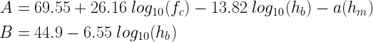
fc = frequency of transmission in MHz, valid range – 150 MHz to 1500 MHz
hb= effective height of transmitting base station antenna in meters, valid range 30 m to 200 m
hm=effective receiving mobile device antenna height in meters, valid range 1m to 10 m
a(hm) = mobile antenna height correction factor that depends on the environment (refer table below)
C = a factor used to correct the formulas for open rural and suburban areas (refer table below)

The function to simulate Hata-Okumura model is given in the book – Wireless Communication Systems using Matlab. The simulated path loss in three types of environments are plotted in Figure 1. The simulated results are obtained over a range of distances for the following parameter values fc=1500 MHz, hb=70 m and hm=1.5 m.

Rate this article: Note: There is a rating embedded within this post, please visit this post to rate it.

References

[1] Masaharu Hata, Empirical formula for propagation loss in land mobile radio services, IEEE transactions on vehicular technology, vol. VT-29, no. 3, August 1980.↗

Topic in this chapter

Books by the author


Wireless Communication Systems in Matlab
Second Edition(PDF)

(173 votes, average: 3.66 out of 5)

Checkout Added to cart

Digital Modulations using Python
(PDF ebook)

(127 votes, average: 3.58 out of 5)

Checkout Added to cart

Digital Modulations using Matlab
(PDF ebook)

(134 votes, average: 3.63 out of 5)

Checkout Added to cart
Hand-picked Best books on Communication Engineering
Best books on Signal Processing

Large scale propagation models – an introduction

Radio propagation models play an important role in designing a communication system for real world applications. Propagation models are instrumental in predicting the behavior of a communication system over different environments. This chapter is aimed at providing the ideas behind the simulation of some of the subtopics in large scale propagation models, such as, free space path loss model, two ray ground reflection model, diffraction loss model and Hata-Okumura model.

This article is part of the book
Wireless Communication Systems in Matlab (second edition), ISBN: 979-8648350779 available in ebook (PDF) format and Paperback (hardcopy) format.

Introduction

Communication over a wireless network requires radio transmission and this is usually depicted as a physical layer in network stack diagrams. The physical layer defines how the data bits are transferred to and from the physical medium of the system. In case of a wireless communication system, such as wireless LAN, the radio waves are used as the link between the physical layer of a transmitter and a receiver. In this chapter, the focus is on the simulation models for modeling the physical aspects of the radio wave when they are in transit.

Radio waves are electromagnetic radiations. The branch of physics that describes the fundamental aspects of radiation is called electrodynamics. Designing a wireless equipment for interaction with an environment involves application of electrodynamics. For example, design of an antenna that produces radio waves, involves solid understanding of radiation physics.

Let’s take a simple example. The most fundamental aspect of radio waves is that it travels in all directions. A dipole antenna, the simplest and the most widely used antenna can be designed with two conducting rods. When the conducting rods are driven with the current from the transmitter, it produces radiation that travels in all directions (strength of radiation will not be uniform in all directions). By applying field equations from electrodynamics theory, it can be deduced that the strength of the radiation field decreases by in the far field, where being the distance from the antenna at which the measurement is taken. Using this result, the received power level at a given distance can be calculated and incorporated in the channel model.

Radio propagation models are broadly classified into large scale and small scale models. Large scale effects typically occur in the order of hundreds to thousands of meters in distance. Small scale effects are localized and occur temporally (in the order of a few seconds) or spatially (in the order of a few meters). This chapter is dedicated for simulation of some of the large-scale models. The small-scale simulation models are discussed in the next chapter.

The important questions in large scale modeling are – how the signal from a transmitter reaches the receiver in the first place and what is the relative power of the received signal with respect to the transmitted power level. Lots of scenarios can occur in large-scale. For example, the transmitter and the receiver could be in line-of-sight in an environment surrounded by buildings, trees and other objects. As a result, the receiver may receive – a direct attenuated signal (also called as line-of-sight (LOS) signal) from the transmitter and indirect signals (or non-line-of-sight (NLOS) signal) due to other physical effects like reflection, refraction, diffraction and scattering. The direct and indirect signals could also interfere with each other. Some of the large-scale models are briefly described here.

The Free-space propagation model is the simplest large-scale model, quite useful in satellite and microwave link modeling. It models a single unobstructed path between the transmitter and the receiver. Applying the fact that the strength of a radiation field decreases as in the far field, we arrive at the Friis free space equation that can tell us about the amount of power received relative to the power transmitted. The log distance propagation model is an extension to Friis space propagation model. It incorporates a path-loss exponent that is used to predict the relative received power in a wide range of environments.

In the absence of line-of-sight signal, other physical phenomena like refection, diffraction, etc.., must be relied upon for the modeling. Reflection involves a change in direction of the signal wavefront when it bounces off an object with different optical properties. The plane-earth loss model is another simple propagation model that considers the interaction between the line-of-sight signal and the reflected signal.

Diffraction is another phenomena in radiation physics that makes it possible for a radiated wave bend around the edges of obstacles. In the knife-edge diffraction model, the path between the transmitter and the receiver is blocked by a single sharp ridge. Approximate mathematical expressions for calculating the loss-due-to-diffraction for the case of multiple ridges were also proposed by many researchers [1][2][3][4].

Of the several available large-scale models, five are selected here for simulation:

Figure 1: Friis free space propagation model (large scale propagation model)

Rate this article: Note: There is a rating embedded within this post, please visit this post to rate it.

References

[1] K. Bullington, Radio propagation at frequencies above 30 megacycles, Proceedings of the IRE, IEEE, vol. 35, issue 10, pp.1122-1136, Oct. 1947.↗

[2] J. Epstein, D. W. Peterson, An experimental study of wave propagation at 850 MC, Proceedings of the IRE, IEEE, vol. 41, issue 5, pp. 595-611, May 1953.↗

[3] J. Deygout, Multiple knife-edge diffraction of microwaves, IEEE Transactions on Antennas Propagation, vol. AP-14, pp. 480-489, July 1966.↗

[4] C.L. Giovaneli, An Analysis of Simplified Solutions for Multiple Knife-Edge Diffraction, IEEE Transactions on Antennas Propagation, Vol. AP-32, No.3, pp. 297-301, March 1984.↗

Topics in this chapter

Books by the author


Wireless Communication Systems in Matlab
Second Edition(PDF)

Note: There is a rating embedded within this post, please visit this post to rate it.
Checkout Added to cart

Digital Modulations using Python
(PDF ebook)

Note: There is a rating embedded within this post, please visit this post to rate it.
Checkout Added to cart

Digital Modulations using Matlab
(PDF ebook)

Note: There is a rating embedded within this post, please visit this post to rate it.
Checkout Added to cart
Hand-picked Best books on Communication Engineering
Best books on Signal Processing