Friis free space propagation model is used to model the line-of-sight (LOS) path loss incurred in a free space environment, devoid of any objects that create absorption, diffraction, reflections, or any other characteristic-altering phenomenon to a radiated wave. It is valid only in the far field region of the transmitting antenna [1] and is based on the inverse square law of distance which states that the received power at a particular distance from the transmitter decays by a factor of square of the distance.
The Friis equation for received power is given by
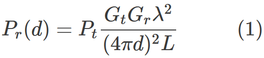
where, Pr is the received signal power in Watts expressed as a function of separation distance (d meters) between the transmitter and the receiver, Pt is the power of the transmitted signal’s Watts, Gt and Gr are the gains of transmitter and receiver antennas when compared to an isotropic radiator with unit gain, λ is the wavelength of carrier in meters and L represents other losses that is not associated with the propagation loss. The parameter L may include system losses like loss at the antenna, transmission line attenuation, loss at various filters etc. The factor L is usually greater than or equal to 1 with L=1 for no such system losses.
[table “36” not found /]
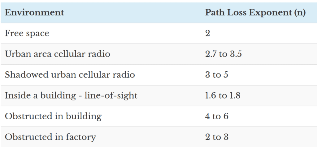
The Friis equation can be modified to accommodate different environments, on the reason that the received signal decreases as the nth power of distance, where the parameter n is the path-loss exponent (PLE) that takes constant values depending on the environment that is modeled (see Table below} for various empirical values for PLE).

The propagation path loss in free space, denoted as PL, is the loss incurred by the transmitted signal during propagation. It is expressed as the signal loss between the feed points of two isotropic antennas in free space.
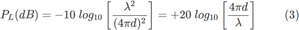
The propagation of an electromagnetic signal, through free space, is unaffected by its frequency of transmission and hence has no dependency on the wavelength λ. However, the variable λ exists in the path loss equation to account for the effective aperture of the receiving antenna, which is an indicator of the antenna’s ability to collect power. If the link between the transmitting and receiving antenna is something other than the free space, penetration/absorption losses are also considered in path loss calculation. Material penetrations are fairly dependent on frequency. Incorporation of penetration losses require detailed analysis.
Usually, the transmitted power and the receiver power are specified in terms of dBm (power in decibels with respect to 1 mW) and the antenna gains in dBi (gain in decibels with respect to an isotropic antenna). Therefore, it is often convenient to work in log scale instead of linear scale. The alternative form of Friis equation in log scale is given by
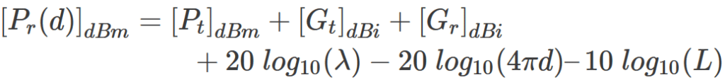
Following function, implements a generic Friis equation that includes the path loss exponent, $latex n$, whose possible values are listed in Table 1.
FriisModel.m: Function implementing Friis propagation model (Refer the book for the Matlab code – click here)
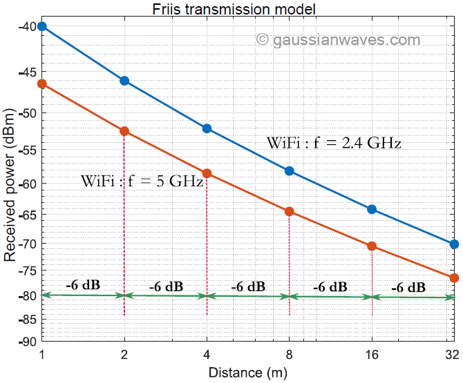
For example, consider a WiFi (IEEE 802.11n standard↗) transmission-reception system operating at f =2.4 GHz or f =5 GHz band with 0 dBm (1 mW) output power from the transmitter. The gain of the transmitter antenna is 1 dBi and that of receiving antenna is 1 dBi. It is assumed that there is no system loss, therefore L = 1. The following Matlab code uses the Friis equation and plots the received power in dBm for a range of distances (Figure 1 shown above). From the plot, the received power decreases by a factor of 6 dB for every doubling of the distance.
Friis_model_test.m: Friis free space propagation model
%Matlab code to simulate Friis Free space equation
%-----------Input section------------------------
Pt_dBm=52; %Input - Transmitted power in dBm
Gt_dBi=25; %Gain of the Transmitted antenna in dBi
Gr_dBi=15; %Gain of the Receiver antenna in dBi
f=110ˆ9; %Transmitted signal frequency in Hertz d =41935000(1:1:200) ; %Array of input distances in meters
L=1; %Other System Losses, No Loss case L=1
n=2; %Path loss exponent for Free space
%----------------------------------------------------
[PL,Pr_dBm] = FriisModel(Pt_dBm,Gt_dBi,Gr_dBi,f,d,L,n);
plot(log10(d),Pr_dBm); title('Friis Path loss model');
xlabel('log10(d)'); ylabel('P_r (dBm)')
Rate this article: [ratings]
References
Books by the author
[table “23” not found /]
I think it’s “Friis”, instead of “Friss”
Thanks for spotting the mistake. Corrected !!!
Free space isotropic propagation is governed by the wave equation, which does not predict that propagation loss is a function of frequency. The Friis equation includes a frequency dependence because it defines Antenna gain relative to an isotropic gain of unity.
see:
https://en.wikipedia.org/wiki/Free-space_path_loss
Path loss can be a function of frequecy if the waves are propagating through an a absorbing media but this is not the assumption for the Friis equation.
Thanks for the eye opener.
In the numerical example, in “…=52 + 2 + 15 +…” , where that 2 came from? if it refers to the transmitter antenna gain, I think it should be 25, not 2. Please clarify. Thanks,
yes. It is a typo in the latex equation. corrected.