Radio propagation models play an important role in designing a communication system for real world applications. Propagation models are instrumental in predicting the behavior of a communication system over different environments. This chapter is aimed at providing the ideas behind the simulation of some of the subtopics in large scale propagation models, such as, free space path loss model, two ray ground reflection model, diffraction loss model and Hata-Okumura model.
[table “36” not found /]
Introduction
Communication over a wireless network requires radio transmission and this is usually depicted as a physical layer in network stack diagrams. The physical layer defines how the data bits are transferred to and from the physical medium of the system. In case of a wireless communication system, such as wireless LAN, the radio waves are used as the link between the physical layer of a transmitter and a receiver. In this chapter, the focus is on the simulation models for modeling the physical aspects of the radio wave when they are in transit.
Radio waves are electromagnetic radiations. The branch of physics that describes the fundamental aspects of radiation is called electrodynamics. Designing a wireless equipment for interaction with an environment involves application of electrodynamics. For example, design of an antenna that produces radio waves, involves solid understanding of radiation physics.
Let’s take a simple example. The most fundamental aspect of radio waves is that it travels in all directions. A dipole antenna, the simplest and the most widely used antenna can be designed with two conducting rods. When the conducting rods are driven with the current from the transmitter, it produces radiation that travels in all directions (strength of radiation will not be uniform in all directions). By applying field equations from electrodynamics theory, it can be deduced that the strength of the radiation field decreases by $latex 1/d$ in the far field, where $latex d$ being the distance from the antenna at which the measurement is taken. Using this result, the received power level at a given distance can be calculated and incorporated in the channel model.
Radio propagation models are broadly classified into large scale and small scale models. Large scale effects typically occur in the order of hundreds to thousands of meters in distance. Small scale effects are localized and occur temporally (in the order of a few seconds) or spatially (in the order of a few meters). This chapter is dedicated for simulation of some of the large-scale models. The small-scale simulation models are discussed in the next chapter.
The important questions in large scale modeling are – how the signal from a transmitter reaches the receiver in the first place and what is the relative power of the received signal with respect to the transmitted power level. Lots of scenarios can occur in large-scale. For example, the transmitter and the receiver could be in line-of-sight in an environment surrounded by buildings, trees and other objects. As a result, the receiver may receive – a direct attenuated signal (also called as line-of-sight (LOS) signal) from the transmitter and indirect signals (or non-line-of-sight (NLOS) signal) due to other physical effects like reflection, refraction, diffraction and scattering. The direct and indirect signals could also interfere with each other. Some of the large-scale models are briefly described here.
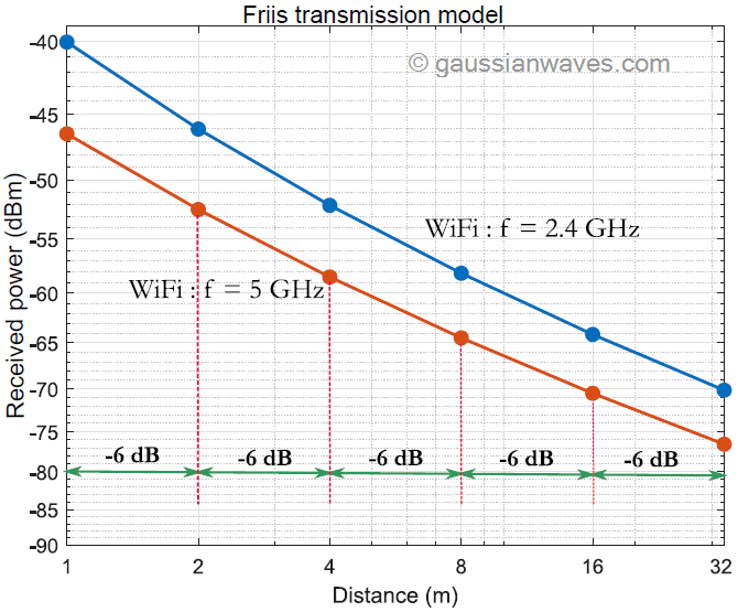
The Free-space propagation model is the simplest large-scale model, quite useful in satellite and microwave link modeling. It models a single unobstructed path between the transmitter and the receiver. Applying the fact that the strength of a radiation field decreases as $latex 1/d$ in the far field, we arrive at the Friis free space equation that can tell us about the amount of power received relative to the power transmitted. The log distance propagation model is an extension to Friis space propagation model. It incorporates a path-loss exponent that is used to predict the relative received power in a wide range of environments.
In the absence of line-of-sight signal, other physical phenomena like refection, diffraction, etc.., must be relied upon for the modeling. Reflection involves a change in direction of the signal wavefront when it bounces off an object with different optical properties. The plane-earth loss model is another simple propagation model that considers the interaction between the line-of-sight signal and the reflected signal.
Diffraction is another phenomena in radiation physics that makes it possible for a radiated wave bend around the edges of obstacles. In the knife-edge diffraction model, the path between the transmitter and the receiver is blocked by a single sharp ridge. Approximate mathematical expressions for calculating the loss-due-to-diffraction for the case of multiple ridges were also proposed by many researchers [1][2][3][4].
Of the several available large-scale models, five are selected here for simulation:
- Friis free space propagation model: to model propagation path loss (Figure 1 shown below)
- Log distance path loss model: incorporates both path loss and shadowing effect
- Two ray ground reflection model, also called as plane-earth loss model
- Single knife-edge diffraction model – incorporates diffraction loss
- Hata – Okumura Model – an empirical model
Rate this article: [ratings]
References
[1] K. Bullington, Radio propagation at frequencies above 30 megacycles, Proceedings of the IRE, IEEE, vol. 35, issue 10, pp.1122-1136, Oct. 1947.↗
[2] J. Epstein, D. W. Peterson, An experimental study of wave propagation at 850 MC, Proceedings of the IRE, IEEE, vol. 41, issue 5, pp. 595-611, May 1953.↗
[3] J. Deygout, Multiple knife-edge diffraction of microwaves, IEEE Transactions on Antennas Propagation, vol. AP-14, pp. 480-489, July 1966.↗
[4] C.L. Giovaneli, An Analysis of Simplified Solutions for Multiple Knife-Edge Diffraction, IEEE Transactions on Antennas Propagation, Vol. AP-32, No.3, pp. 297-301, March 1984.↗
Topics in this chapter
- Introduction to Large scale propagation models
- Friis free space propagation model
- Log distance path loss model
- Two ray ground reflection model
- Modeling diffraction loss
- Hata Okumura model for outdoor propagation
Books by the author
[table “23” not found /]