Tag: sinc function

Numerous texts are available to explain the basics of Discrete Fourier Transform and its very efficient implementation – Fast Fourier Transform (FFT).  Often we are confronted with the need to generate simple, standard signals (sine, cosine, Gaussian pulse, square wave, isolated rectangular pulse, exponential decay, chirp signal) for simulation purpose. I intend to show (in a series of articles) how these basic signals can be generated in Matlab and how to represent them in frequency domain using FFT.

This article is part of the book Digital Modulations using Matlab : Build Simulation Models from Scratch, ISBN: 978-1521493885 available in ebook (PDF) format (click here) and Paperback (hardcopy) format (click here)
Wireless Communication Systems in Matlab, ISBN: 978-1720114352 available in ebook (PDF) format (click here) and Paperback (hardcopy) format (click here).

Rectangular pulse: mathematical description

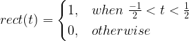
An isolated rectangular pulse of amplitude A and duration T is represented mathematically as

where

The Fourier transform of isolated rectangular pulse g(t) is

where, the sinc function is given by

Thus, the Fourier Transform pairs are

The Fourier Transform describes the spectral content of the signal at various frequencies. For a given signal g(t), the Fourier Transform is given by

where, the absolute value gives the magnitude of the frequency components (amplitude spectrum) and are their corresponding phase (phase spectrum) . For the rectangular pulse, the amplitude spectrum is given as

The amplitude spectrum peaks at f=0 with value equal to AT. The nulls of the spectrum occur at integral multiples of 1/T, i.e, ( )

Generating an isolated rectangular pulse in Matlab:

An isolated rectangular pulse of unit amplitude and width w (the factor T in equations above ) can be generated easily with the help of in-built function – rectpuls(t,w) command in Matlab. As an example, a unit amplitude rectangular pulse of duration is generated.

fs=500; %sampling frequency
T=0.2; %width of the rectangule pulse in seconds

t=-0.5:1/fs:0.5; %time base

x=rectpuls(t,T); %generating the square wave

plot(t,x,'k');
title(['Rectangular Pulse width=', num2str(T),'s']);
xlabel('Time(s)');
ylabel('Amplitude');

Amplitude spectrum using FFT:

Matlab’s FFT function is utilized for computing the Discrete Fourier Transform (DFT). The magnitude of FFT is plotted. From the following plot, it can be noted that the amplitude of the peak occurs at f=0 with peak value  . The nulls in the spectrum are located at  ().

L=length(x);
NFFT = 1024;
X = fftshift(fft(x,NFFT)); %FFT with FFTshift for both negative & positive frequencies
f = fs*(-NFFT/2:NFFT/2-1)/NFFT; %Frequency Vector

figure;
plot(f,abs(X)/(L),'r');
title('Magnitude of FFT');
xlabel('Frequency (Hz)')
ylabel('Magnitude |X(f)|');

Power spectral density (PSD) using FFT:

The distribution of power among various frequency components is plotted next. The first plot shows the double-side Power Spectral Density which includes both positive and negative frequency axis. The second plot describes the PSD only for positive frequency axis (as the response is just the mirror image of negative frequency axis).

figure;
Pxx=X.*conj(X)/(L*L); %computing power with proper scaling
plot(f,10*log10(Pxx),'r');
title('Double Sided - Power Spectral Density');
xlabel('Frequency (Hz)')
ylabel('Power Spectral Density- P_{xx} dB/Hz');

X = fft(x,NFFT);
X = X(1:NFFT/2+1);%Throw the samples after NFFT/2 for single sided plot
Pxx=X.*conj(X)/(L*L);
f = fs*(0:NFFT/2)/NFFT; %Frequency Vector
plot(f,10*log10(Pxx),'r');
title('Single Sided - Power Spectral Density');
xlabel('Frequency (Hz)')
ylabel('Power Spectral Density- P_{xx} dB/Hz');

Magnitude and phase spectrum:

The phase spectrum of the rectangular pulse manifests as series of pulse trains bounded between 0 and , provided the rectangular pulse is symmetrically centered around sample zero. This is explained in the reference here and the demo below.

clearvars;
x = [ones(1,7) zeros(1,127-13) ones(1,6)];
subplot(3,1,1); plot(x,'k');
title('Rectangular Pulse'); xlabel('Sample#'); ylabel('Amplitude');

NFFT = 127;
X = fftshift(fft(x,NFFT)); %FFT with FFTshift for both negative & positive frequencies
f = (-NFFT/2:NFFT/2-1)/NFFT; %Frequency Vector

subplot(3,1,2); plot(f,abs(X),'r');
title('Magnitude Spectrum'); xlabel('Frequency (Hz)'); ylabel('|X(f)|');

subplot(3,1,3); plot(f,atan2(imag(X),real(X)),'r');
title('Phase Spectrum'); xlabel('Frequency (Hz)'); ylabel('\angle X(f)');

Rate this article: Note: There is a rating embedded within this post, please visit this post to rate it.

Topics in this chapter

Essentials of Signal Processing ● Generating standard test signals  □ Sinusoidal signals  □ Square wave  □ Rectangular pulse  □ Gaussian pulse  □ Chirp signal ● Interpreting FFT results - complex DFT, frequency bins and FFTShift  □ Real and complex DFT  □ Fast Fourier Transform (FFT)  □ Interpreting the FFT results  □ FFTShift  □ IFFTShift ● Obtaining magnitude and phase information from FFT  □ Discrete-time domain representation  □ Representing the signal in frequency domain using FFT  □ Reconstructing the time domain signal from the frequency domain samples ● Power spectral density ● Power and energy of a signal  □ Energy of a signal  □ Power of a signal  □ Classification of signals  □ Computation of power of a signal - simulation and verification ● Polynomials, convolution and Toeplitz matrices  □ Polynomial functions  □ Representing single variable polynomial functions  □ Multiplication of polynomials and linear convolution  □ Toeplitz matrix and convolution ● Methods to compute convolution  □ Method 1: Brute-force method  □ Method 2: Using Toeplitz matrix  □ Method 3: Using FFT to compute convolution  □ Miscellaneous methods ● Analytic signal and its applications  □ Analytic signal and Fourier transform  □ Extracting instantaneous amplitude, phase, frequency  □ Phase demodulation using Hilbert transform ● Choosing a filter : FIR or IIR : understanding the design perspective  □ Design specification  □ General considerations in design

Books by the author

Wireless Communication Systems in Matlab Second Edition(PDF) Note: There is a rating embedded within this post, please visit this post to rate it. $14.99 – Add to Cart Checkout Added to cart	Digital Modulations using Python (PDF ebook) Note: There is a rating embedded within this post, please visit this post to rate it. $14.99 – Add to Cart Checkout Added to cart	Digital Modulations using Matlab (PDF ebook) Note: There is a rating embedded within this post, please visit this post to rate it. $14.99 – Add to Cart Checkout Added to cart
Hand-picked Best books on Communication Engineering Best books on Signal Processing