Key focus: “Why can’t I just use a matrix to solve ARMA?” The answer is right there in the shape of the surface—you can’t solve a “warped” landscape with a linear equation.
Introduction
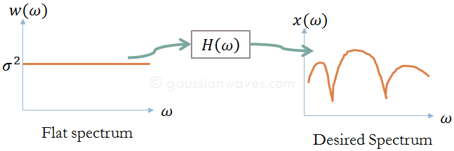
In signal modeling, our goal is to find a set of coefficients (ak and bk) that best describe an observed signal. We do this by minimizing the Prediction Error—the difference between the actual signal and what our model predicts.
However, as we move from the simple Auto-Regressive (AR) model to the generalized Auto-Regressive Moving Average (ARMA) model, we move from a straightforward mathematical problem to a complex numerical nightmare. Here is why.
The AR Model: A Predictable Linear Path
In an AR model, we predict the current sample $x[n]$ using only past samples of the output. The difference between the actual sample and our prediction is the error w[n] (often treated as the driving white noise):
$$w[n]=x[n]−\left(−\sum_{k=1}^{N}a_kx[n−k] \right)$$
Why it’s easy to solve:
To find the optimal coefficients $a_k$, we minimize the Sum of Squared Errors (SSE): $E= \sum w^2[n]$.
- Quadratic Nature: The error w[n] is a linear function of the parameters $a_k$. This means the squared error $E$ is a quadratic function.
- Unique Minimum: Quadratic functions are “bowl-shaped.” They have a single, global minimum. We can find this minimum analytically by taking the derivative and setting it to zero, leading to the famous Yule-Walker equations (linear matrix algebra).
As discussed in the previous post, the ARMA model is a generalized model that is a mix of both AR and MA model. Given a signal x[n], AR model is easiest to find when compared to finding a suitable ARMA process model. Let’s see why this is so.
The ARMA Model: The Non-Linear Trap
The ARMA model is more powerful because it uses both past outputs ($a_k$) and past inputs/errors ($b_k$) to predict the current sample:
$$w[n]=x[n]−\left(− \sum_{k=1}^{N} a_k x[n−k]+ \sum_{k=1}^{M} b_k w[n−k] \right)$$
Why it’s difficult to solve:
Look closely at the term $\sum b_k w[n−k]$. This is where the trouble starts.
- The Recursive Feedback: To calculate the current error w[n], you need to know the previous errors $w[n−k]$. But those previous errors themselves depend on the unknown coefficients $b_k$.
- Non-Linearity: Because $w[n]$ is now a function of $b_k$ multiplied by previous $w$ terms (which also contain $b_k$), the error becomes non-linear with respect to the parameters.
- No Unique Solution: The Squared Error surface for an ARMA model is no longer a simple bowl. It is a “rugged landscape” with multiple local minima, plateaus, and valleys.
The Numerical Headache: You cannot solve ARMA coefficients with a single matrix inversion. Instead, you must use iterative numerical optimization (like Gauss-Newton or Levenberg-Marquardt), which can get stuck in the “wrong” local minimum or fail to converge entirely.
To visualize why ARMA is so much harder to solve, we can use Python to map the “Error Surface.” For a simple AR model, this surface is a perfect, convex bowl. For an ARMA model, the surface becomes warped, often showing multiple valleys where an optimizer could get stuck.
Python: ARMA Error Surface Visualization
This script simulates an ARMA(1,1) process and then calculates the Sum of Squared Errors (SSE) for a grid of possible $a_1$ and $b_1$ values.
import numpy as np
import matplotlib.pyplot as plt
from scipy import signal

# 1. Generate "True" Data using ARMA(1,1)
# x[n] = -a1*x[n-1] + w[n] + b1*w[n-1]
true_a1, true_b1 = -0.5, 0.4
n_samples = 500
white_noise = np.random.randn(n_samples)
x = signal.lfilter([1, true_b1], [1, true_a1], white_noise)

# 2. Define the Search Grid for parameters
a_range = np.linspace(-0.9, 0.9, 50)
b_range = np.linspace(-0.9, 0.9, 50)
A, B = np.meshgrid(a_range, b_range)
sse_surface = np.zeros(A.shape)

# 3. Calculate SSE for every point in the grid
for i in range(len(a_range)):
    for j in range(len(b_range)):
        # Inverse filter to find the residuals (errors)
        # w[n] = x[n] + a*x[n-1] - b*w[n-1]
        errors = signal.lfilter([1, a_range[i]], [1, b_range[j]], x)
        sse_surface[j, i] = np.sum(errors**2)

# 4. Plotting the Error Surface
fig = plt.figure(figsize=(12, 8))
ax = fig.add_subplot(111, projection='3d')
surf = ax.plot_surface(A, B, sse_surface, cmap='viridis', antialiased=True)

ax.set_title('SSE Error Surface for ARMA(1,1)')
ax.set_xlabel('AR Parameter (a1)')
ax.set_ylabel('MA Parameter (b1)')
ax.set_zlabel('Sum of Squared Errors')
fig.colorbar(surf, shrink=0.5, aspect=5)
plt.show()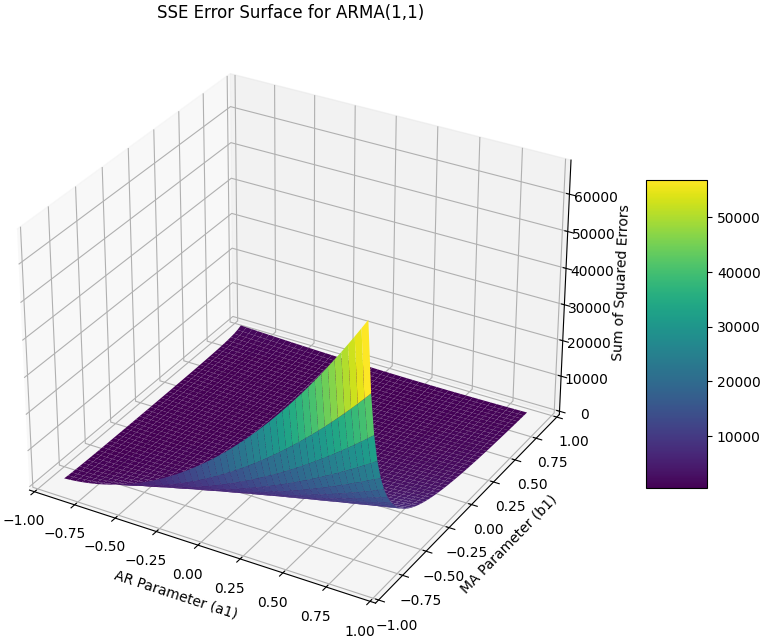
Understanding the Visualization
When you run this or look at the resulting plot, notice these specific features:
- The Non-Convexity: Unlike the AR model, which produces a “parabolic bowl” with a single, clear bottom, the ARMA surface is non-linear. The error is “recursively” coupled—meaning that as you change b1, the entire history of the errors changes.
- The Optimization Challenge: If you start a numerical optimizer (like Gradient Descent) on a high “ridge” of this surface, it might fall into a local minimum that isn’t the true global minimum (the “true” parameters of our signal).
- The Convergence Problem: Near the edges of the grid (where poles or zeros approach the unit circle), the error spikes toward infinity. This is why ARMA solvers often crash or fail to converge if the initial guess is poor.
Summary Comparison
| Feature | AR Model (All-Pole) | ARMA Model (Pole-Zero) |
| Error Function | Linear w.r.t parameters | Non-linear w.r.t parameters |
| Error Surface | Quadratic (Simple Bowl) | Non-Quadratic (Rugged) |
| Optimization | Analytic (Linear Algebra) | Iterative (Numerical Methods) |
| Solution | Unique Global Minimum | Multiple Local Minima Possible |
Engineering Insight
This is why engineers often prefer high-order AR models even when an ARMA model might theoretically be more “compact.” A high-order AR model might require more coefficients, but it guarantees a stable, unique, and easily calculated solution. ARMA is the “high-performance” engine that is notoriously difficult to tune.
References
[1] G. Thiesson, C. Meek, and D. Chickering, “ARMA time series modeling with graphical models,” in Proc. 20th Conf. Uncertainty in Artif. Intell. (UAI), Banff, Canada, Jul. 2004, pp. 552–560.
[2] S. M. Kay, Fundamentals of Statistical Signal Processing: Estimation Theory. Upper Saddle River, NJ, USA: Prentice-Hall, 1993.
[3] J. G. Proakis and D. G. Manolakis, Digital Signal Processing: Principles, Algorithms, and Applications, 4th ed. Upper Saddle River, NJ, USA: Pearson Prentice Hall, 2007.
[4] G. E. P. Box, G. M. Jenkins, G. C. Reinsel, and G. M. Ljung, Time Series Analysis: Forecasting and Control, 5th ed. Hoboken, NJ, USA: Wiley, 2015.