A practical, hands‑on mini‑guide for DSP engineers moving Matlab workflows to Python. Includes a conversion checklist, runnable examples (filter design, spectrogram), tool recommendations, and troubleshooting tips.
TL;DR Matlab and Python both excel for DSP. To migrate safely: identify inputs/outputs, map built‑ins to SciPy/NumPy, fix indexing and shape, convert plotting, add tests and example data, and run comparisons. Use Jupyter/Colab for reproducibility and GitHub for distribution.
Introduction
Moving a DSP workflow from Matlab to Python doesn’t have to be painful — it’s an opportunity. Matlab has long been the go‑to for signal processing research and prototyping, but Python’s open ecosystem (NumPy, SciPy, Matplotlib), cloud‑friendly notebooks, and seamless integration with modern ML tool chains make it the pragmatic choice for reproducible research and production deployment. This mini‑guide gives you a practical, low‑risk path to migrate your Matlab scripts and toolboxes into readable, testable Python code you can run in Jupyter/Colab.
You’ll learn how to inventory inputs and baseline outputs, map common Matlab built‑ins to SciPy/NumPy equivalents, and avoid the usual pitfalls around 1‑based indexing, array shapes, and plotting differences. More importantly, the guide emphasizes verification: saving Matlab baselines, writing pytest checks, and comparing numeric and visual results so you can prove parity rather than guessing. Each concept includes runnable examples — a FIR filter design and a spectrogram demo — with ready‑to‑run Colab notebooks.
If you’re keeping legacy Matlab code for experiments but want the flexibility of Python, this guide walks you step‑by‑step from conversion checklist to validated notebooks and CI‑ready tests. Start with the TL;DR checklist or jump straight to the examples to run them in Colab.
Why move
- Python is free, widely used, and has a strong ecosystem (NumPy, SciPy, Matplotlib, Jupyter).
- Easier deployment to production and to cloud (Colab, Docker).
- Better integration with ML libraries (PyTorch, TensorFlow) for modern DSP+AI workflows.
Conversion checklist (step‑by‑step)
- Inventory: list Matlab scripts, functions, and toolboxes used. Mark high‑priority items.
- Data: collect or generate a small test dataset and expected outputs (MAT files, plots).
- Map functions: identify Matlab built‑ins and find Python equivalents (see mappings below).
- Convert numerics: translate matrix/vector code and fix indexing (Remember: Matlab uses
1..Nfor indices). - Replace plotting: switch Matlab plotting to Matplotlib/Plotly (preserve figure look if needed).
- Validate: write unit tests or notebooks that compare results (arrays close within tolerance).
- Package: place scripts in a GitHub repo with a README and a Colab notebook.
- Optional: optimize performance with NumPy broadcasting, Numba, or Cython if needed.
Inventory inputs & outputs
Know exactly what your Matlab code consumes and produces so you can validate equivalence. Reproducible inputs + baseline outputs let you prove parity quickly instead of eyeballing plots.
- List input file formats (WAV, MAT, CSV), parameters (fs, N, window), and expected outputs (plots, arrays, MAT files).
- Create a tiny, canonical test dataset you can reuse for comparisons (e.g., a short synthetic signal or a saved MAT file).
- Save Matlab baseline outputs: numeric arrays and a few scalar metrics (peak magnitude, RMS, SNR, BER) into a
.matusingsave('baseline.mat','var1','var2',...).
Map Matlab built‑ins to SciPy/NumPy (and other Python libs)
- Matrix & arrays: Matlab arrays → NumPy arrays (import numpy as np)
- Signal processing: Matlab functions (butter, fir1, freqz, spectrogram) → scipy.signal (butter, firwin, freqz, spectrogram)
- FFT:
fft, ifft → np.fft.fft, np.fft.ifft - Loading/saving: load/save MAT files →
scipy.io.loadmat/savematorh5pystoragefor v7.3 (Note: The Python packagehdf5storageis a robust solution for reading and writing HDF5 files that are fully compatible with MATLAB v7.3 files. It handles the necessary data conversions automatically.) - Plotting:
plot, subplot→matplotlib.pyplot - Scripts → modules: wrap long scripts in functions for testability
Key conversion pitfalls and how to handle them
- Core difference: Matlab is 1‑based and uses 2D arrays (column vs row vectors); NumPy is 0‑based and uses 1D arrays for vectors.
- Example pitfall:
x = a(:,1)in Matlab yields a column vector;a[:,0]in Python returns a 1D array — usea[:,0:1]to keep 2D.
- Example pitfall:
- Indexing: Subtract 1 from any hard-coded indices in loops or referencing (e.g.,
x(1:N)→x[0:N]). - Shape: Matlab distinguishes column vs row by default. In NumPy, vectors are 1D unless explicitly reshaped—use
.reshape((-1,1))when needed. - Use
.copy()when you need explicit copies (Matlab often behaves like copy-on-write). - Complex numbers: Matlab stores complex arrays; NumPy handles them but ensure
dtype (np.complex128). - Function names and parameter orders change: check docstrings; for example, SciPy’s
freqzparameter order differs. - Toolboxes: if you used Matlab toolboxes (e.g., Signal Processing, Communications), search for Python alternatives (
scipy.signal, commpy, pyradioml) or implement missing pieces manually.
Convert plotting and preserve readability
- Map:
plot,subplot,imagesc,surf→ Matplotlib (or Plotly for interactivity). - Recreate common Matlab behaviors:
imagesc→plt.imshow(..., aspect='auto', origin='lower')orpcolormesh.mesh/surf→mpl_toolkits.mplot3dor Plotlygo.Surface.
- Keep a short “plotting style” snippet to match Matlab visuals (fonts, grid, axis limits).
- Example: replace Matlab’s colormap defaults or axis orientation if results look flipped.
Add tests and example data (validation)
Minimal test strategy:
- Save Matlab baseline arrays as
baseline.mat. For each converted Python function, load the baseline and compare:- Numeric arrays:
np.allclose(py_out, matlab_out, atol=1e-9, rtol=1e-6)— choose tolerances appropriate to algorithm (floating point, filter states). - Scalar metrics: compare with absolute tolerances (e.g., peak error < 1e-6 or relative error < 1e-3).
- Numeric arrays:
- Visual checks: compute scalar summaries of plots (peak frequency, centroid) and compare numerically rather than comparing images.
Run comparisons (numeric + visual)
- Numeric parity: compare arrays, spectral peaks, energy, SNR, BER curves.
- Visual parity: compute metrics derived from the visual (e.g., peak magnitude, dominant frequency) and compare numbers rather than pixels.
- Tolerances: expect small floating point deviations. For filters, compare frequency responses at identical frequency bins and compute max dB difference.
Testing & validation
- Create a small test suite using
pytestthat loads the Matlab output (saved via.mat) and compares results with NumPy usingnp.allclose(..., atol=1e-6). - Example test outline:
- Input stimuli → run Matlab (baseline) → save numeric outputs.
- Convert Python → run Python on same stimuli → compare arrays and plots (peak values, RMS error).
- For plots: compare derived scalar metrics (e.g., peak magnitude, center frequency) rather than pixel‑by‑pixel images unless you use image comparison tools.
Tooling & recommended libraries for Python
- Core: numpy, scipy, matplotlib, jupyter, pandas (for tabular data)
- Audio: soundfile, librosa (audio analysis)
- DSP helpers: scipy.signal, commpy (community), pyradioml (radio/ML)
- Notebook/Cloud: jupyter, Google Colab (shareable)
- Performance: numba, Cython, pybind11 (for C++ integration)
- Packaging: pipenv/venv, poetry, requirements.txt or pyproject.toml
Example 1: FIR lowpass design and frequency response
Matlab (original)
Notes
- Matlab fir1’s default window differs from
firwindefaults; choose window parameter to match (e.g.,'hamming'). - Matlab’s
(H, w); Vs. SciPy’sfreqzreturns(w, H)– check the order. - After computing
[H,w], the script saves the output data & variables needed for test & validation in python
fs = 1000;                % sampling frequency
fc = 100;                 % cutoff freq
N = 51;                   % filter length (odd)
wn = fc/(fs/2);           % normalized freq
b = fir1(N-1, wn, 'low'); % FIR design
[H, w] = freqz(b,1,512,fs);
plot(w, 20*log10(abs(H)));
xlabel('Frequency (Hz)');
ylabel('Magnitude (dB)');
title('FIR Lowpass Frequency Response');


% Save baseline for use by pytest (variables: b, fs, w, H)
save('baseline_fir_lowpass.mat', 'b', 'fs', 'w', 'H');
fprintf('Saved baseline to baseline_fir_lowpass.mat\n');Python (NumPy/SciPy/Matplotlib equivalent)
Here is the runnable python code. Click Run and see the result below. The same code is available in Google Colab for you to explore.
Simulated Result
Writing Test & Validation in Python
Now that we have stored the expected baseline from Matlab script and the python script for computing the Lowpass FIR design is also available, the next step is to test and validate the output in python. We will verify whether the Python implementation match MATLAB baseline for FIR lowpass design.
Following script requires the use of pytest library in python. If you do not have one, install it using the following command.
pip install pytestFor installing in Google colab
!pip install pytestFollowing test script checks that the Python FIR design and frequency-response code reproduces the MATLAB result numerically (not just visually).
# test_fir_lowpass.py
import os
import numpy as np
import pytest
import hdf5storage
from firLowpass import compute_fir_lowpass


def test_fir_lowpass_matches_baseline():
    """Minimal test: load baseline and compare w/H to compute_fir_lowpass output."""
    baseline = os.path.join('.', 'baseline_fir_lowpass.mat')
    if not os.path.exists(baseline):
        pytest.skip('Baseline not found; run fir_lowpass.m in MATLAB or generate baseline')

    data = hdf5storage.loadmat(baseline)
    if 'w' not in data or 'H' not in data:
        pytest.skip('Baseline missing w/H')

    w_mat = np.asarray(data['w']).squeeze()
    H_mat = np.asarray(data['H']).squeeze()

    w_py, H_py, _ = compute_fir_lowpass(plot=False)

    assert np.allclose(w_py, w_mat, atol=1e-6), 'Frequency vectors differ'
assert np.allclose(H_py, H_mat, atol=1e-6), 'Frequency responses differ'Run the test
pytest -v test_fir_lowpass.pyTest result:
(.venv) PS > pytest -v test_fir_lowpass.py
============= test session starts ==========================
platform -- Python 3.12.2, pytest-8.4.2, pluggy-1.6.0 -- python.exe
collected 1 item

test_fir_lowpass.py::test_fir_lowpass_matches_baseline PASSED                                                              [100%]

========= 1 passed in 1.46s ===============================Example 2: Spectrogram
Matlab (original)
% Clear workspace and command window
clear;
clc;

%Load the variables from handel.mat
data = load('handel.mat'); %Replace with your file
audioSignal = data.y;
sampleFrequency = data.Fs;

% Define spectrogram parameters
windowLength = 256; % Length of the window in samples
noverlap = round(0.75 * windowLength); % Overlap between segments (e.g., 75%)
nfft = max(256, 2^nextpow2(windowLength)); % Number of DFT points for FFT

% Compute and plot the spectrogram
figure;
[Sxx,frequencies,times] = spectrogram(audioSignal, windowLength, noverlap, nfft, sampleFrequency);

% Calculate the data to be plotted
eps = 1e-12;
data_to_plot = 10 * log10(abs(Sxx) + eps);

% Use imagesc for plotting
imagesc(times, frequencies, data_to_plot);

% Ensure correct axis orientation
axis xy;
% Apply shading interpolation (equivalent to using it with pcolor)
shading interp;
% Add a colorbar for reference
colorbar;

title('Spectrogram of the Signal');
xlabel('Time (s)');
ylabel('Frequency (Hz)');

% Ensure y-axis shows Hz up to Nyquist (Fs/2)
ylim([0 sampleFrequency/2]);
Python (NumPy/SciPy/Matplotlib equivalent)
import numpy as np
import hdf5storage
#await micropip.install('hdf5storage');
import matplotlib.pyplot as plt
#import matplotlib
from scipy import signal

# matplotlib backend needed with inseri-core
#matplotlib.use('Agg')

# Load the variables from the .mat file using hdf5storage
try:
    data = hdf5storage.loadmat('handel.mat') #replace with your file
    audio_signal = data['y']
    sample_frequency = data['Fs']
except FileNotFoundError:
    print("Error: 'handel.mat' not found. Please ensure the file is in the correct directory.")
    exit()

# Flatten the audio signal if it's not a 1D array
if audio_signal.ndim > 1:
    audio_signal = audio_signal.flatten()

# Define spectrogram parameters
window_length = 256
noverlap = round(0.75 * window_length)
nfft = max(256, 2**(int(np.ceil(np.log2(window_length)))))

# Compute the spectrogram
frequencies, times, Sxx = signal.spectrogram(audio_signal, fs=sample_frequency,
                                             window='hamming', nperseg=window_length,
                                             noverlap=noverlap, nfft=nfft,
                                             scaling='spectrum', mode='complex')

# Calculate the data to be plotted
eps = np.finfo(float).eps
data_to_plot = 10 * np.log10(np.abs(Sxx) + eps)

# Create and configure the plot
plt.figure(figsize=(10, 6))

# Fix the extent parameter to use min/max values
plt.imshow(data_to_plot, origin='lower', aspect='auto',
           extent=[times.min(), times.max(), frequencies.min(), frequencies.max()])

# Add a colorbar for reference
plt.colorbar(label='Magnitude (dB)')

# Set plot labels and title
plt.title('Spectrogram of the Signal')
plt.xlabel('Time (s)')
plt.ylabel('Frequency (Hz)')

# Ensure y-axis shows Hz up to the Nyquist frequency (Fs/2)
plt.ylim([0, sample_frequency / 2])

plt.savefig("img.png", format='png', bbox_inches='tight')
plt.close()
# To display the plot plt.show()Results comparison
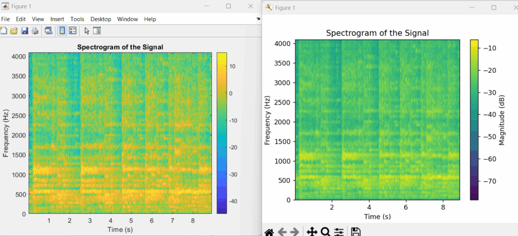
Test & Validation
Replicating MATLAB spectrogram in Python requires manually matching the specific parameters, as their defaults differ significantly. This includes the window type and length, segment overlap, FFT length, and output scaling. The core reason for fundamental differences between MATLAB’s spectrogram and Python’s scipy.signal.spectrogram is their different default parameter choices, output types, and underlying Fast Fourier Transform (FFT) algorithms. These functions are tools within entirely separate software ecosystems and are not designed to be identical out-of-the-box.
With this, a practical hands-on guide for moving work flows from Matlab to python is demonstrated. Now its time for you to explore further.