Array pattern multiplication of phased array antennas

Key focus: Array pattern multiplication: total radiation pattern of N identical antennas is product of single-antenna radiation vector and array factor.

Antenna arrays

Ferdinand Braun invented the Phased Array Antenna in 1905. He shared a Nobel Prize in physics in recognition of their contributions to the development of wireless telegraphy.

An antenna array is a collection of numerous linked antenna elements that operate together to broadcast or receive radio waves as if they were a single antenna. Phased array antennas are used to focus the radiated power towards a particular direction. The angular pattern of the phased array depends on the number of antenna elements, their geometrical arrangement in the array, and relative amplitudes and phases of the array elements.

Phased array antennas can be used to steer the radiated beam towards a particular direction by adjusting the relative phases of the array elements.

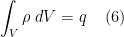
The basic property of antenna arrays is the translational phase-shift.

Time-shift property of Fourier transform

Let’s focus for a moment on the time-shifting property of Fourier transform. The timeshifting property implies that a shift in time corresponds to a phase rotation in the frequency domain.

\[F \left\{x(t−t_0) \right\}=e^{-j \omega t_0}X(\omega) \quad \quad (1)\]

Translational phase-shift property

Now, let’s turn our attention to antenna elements translated/shift in space. Figure 1 depicts a single antenna element having current density J(r) placed at the origin is moved in space to a new location that is l0 distant from the original position. The current density of the antenna element at the new position l0 is given by

\[J_{l_0}(r) = J(r – l_0) \quad \quad (2)\]
Figure 1: Current density of antenna element shifted in space

From the discussion on far-field retarded potentials, the radiation vector F(θ,ɸ) of an antenna element is given by the three dimensional spatial Fourier transform of current density J(z).

\[\mathbf{F} \left(\mathbf{k} \right) =\int_V J(r)e^{j \mathbf{k} \cdot r } d^3 r, \quad \quad \mathbf{k} = k\hat{r} \quad \quad (3) \]

Therefore, from equations (2) and (3), the radiation vector of the antenna element space-shifted to new position l0 is given by the space shift property (similar to time-shift property of Fourier transform in equation (1))

\[\begin{aligned} \mathbf{F}_{l_0} \left(\mathbf{k} \right) &=\int_V J_{l_0}(r)e^{j \mathbf{k} \cdot r } d^3 r \\ &= \int_V J(r-l_0)e^{j \mathbf{k} \cdot r } d^3 r \\ &= \int_V J(r)e^{j \mathbf{k} \cdot (r+l_0) } d^3 r \\ &= e^{j \mathbf{k} l_0}\int_V J(r)e^{j \mathbf{k} \cdot r } d^3 r \\ &= e^{j \mathbf{k} l_0} \mathbf{F} \left(\mathbf{k} \right) \end{aligned} \\ \Rightarrow \boxed{ \mathbf{F}_{l_0} \left(\mathbf{k} \right) = e^{j \mathbf{k} l_0} \mathbf{F}\left(\mathbf{k} \right) } \quad \quad (4) \]

Note: The sign of exponential in the Fourier transform does not matter (it just indicates phase rotation in opposite direction), as long as the same convention is used throughout the analysis.

From equation (4), we can conclude that the relative location of the antenna elements with regard to one another causes relative phase changes in the radiation vectors, which can then contribute constructively in certain directions or destructively in others.

Array factor and array pattern multiplication

Figure 2 depicts a more generic case of identical antenna elements placed in three dimensional space at various radial distances l0, l1, l2, l3, … and the antenna feed coefficients respectively are a0, a1, a2, a3,…

Figure 2: Current densities of antenna elements shifted in space – contributors to array factor of phased array antenna

The current densities of the individual antenna elements are

\[\begin{aligned} J_{l_0}(r) &= a_0 J(r – l_0) \\ J_{l_1}(r) &= a_1 J(r – l_1) \\ J_{l_2}(r) &= a_2 J(r – l_2) \\ & \vdots \end {aligned} \quad \quad (5)\]

The total current density of the antenna array structure is

\[J_{total} = a_0 J(r – l_0) + a_1 J(r – l_1) + a_2 J(r – l_2) + \cdots \quad \quad (6)\]

Applying the translational phase-shift property in equation (4), the total radiation vector of an N element antenna array is given by

\[ \begin{aligned} \mathbf{F}_{total} \left(\mathbf{k} \right) &=\mathbf{F}_{l_0} \left(\mathbf{k} \right) + \mathbf{F}_{l_1} \left(\mathbf{k} \right) + \mathbf{F}_{l_2} \left(\mathbf{k} \right) + \cdots \\ &= a_0 e^{j \mathbf{k} l_0} \mathbf{F} \left(\mathbf{k} \right) + a_1 e^{j \mathbf{k} l_1} \mathbf{F} \left(\mathbf{k} \right) + a_2 e^{j \mathbf{k} l_2} \mathbf{F} \left(\mathbf{k} \right) + \cdots\\ &= \mathbf{F} \left(\mathbf{k} \right) \sum_{i=0}^{N} a_i e^{j \mathbf{k} l_i} \\ &= \mathbf{F} \left(\mathbf{k} \right) \mathbf{A} \left(\mathbf{k} \right)\end{aligned} \]
\[ \boxed{\mathbf{F}_{total} \left(\mathbf{k} \right) = \mathbf{F} \left(\mathbf{k} \right) \mathbf{A} \left(\mathbf{k} \right) \quad \quad (\text{array pattern multiplication}) } \quad \quad (7)\]

The quantity A(k) is called array factor which incorporates the relative translational phase shifts and the relative feed coefficients of the array elements.

\[\boxed{\mathbf{A} \left(\mathbf{k} \right) = \sum_{i=0}^{N} a_i e^{j \mathbf{k} l_i} \quad \quad (\text{array factor}) }\quad \quad ,\mathbf{k} = k\hat{r} \quad \quad (8)\]

or equivalently,

\[\boxed{\mathbf{AF} \left(\theta, \phi \right) = \sum_{i=0}^{N} a_i e^{j k \left( \hat{\theta} \times \hat{\phi} \right) l_i} \quad \quad (\text{array factor}) } \quad \quad (9)\]

The array pattern multiplication property states that the total radiation pattern of an antenna array constructed with N identical antennas is the product of radiation vector of a single individual antenna element (also called as element factor) and the array factor.

Effect of array factor on power gain and radiation intensity

Let U(θ,ɸ) and G(θ,ɸ) denote the radiation intensity and the power gain patterns of an antenna element. The total radiation intensity and the power gain of an antenna array, constructed with such identical antenna elements, will be modified by the array factor as follows.

\[\boxed{\begin{aligned} U_{total}\left( \theta, \phi \right) &= \mid A(\theta, \phi)\mid ^2 U\left( \theta, \phi \right)\\ G_{total}\left( \theta, \phi \right) &= \mid A(\theta, \phi)\mid ^2 G\left( \theta, \phi \right) \end{aligned}} \quad \quad (10)\]

The role of array factor is very similar to that of the transfer function of an linear time invariant system. Recall that if a wide sense stationary process x(t) is input to the LTI system defined by the transfer function H(f), then the power spectral density of the output is given by

\[S_y(f) = \mid H(f) \mid ^2 S_x(f)\]

Illustration using a linear array of half-wave dipole antennas

Linear antennas are electrically thin antennas whose conductor diameter is very small compared to the wavelength of the radiation λ.

A linear antenna oriented along the z-axis has radiation vector (field) whose components are along the directions of the radial distance and the polar angle. That is, the radiation intensity U(θ,ɸ) and the power gain G(θ,ɸ) depend only on the polar angle θ. In other words, the radiation intensity and the power gain are omnidirectional (independent of azimuthal angle ɸ).

Figure 3, illustrates an antenna array with linear half-wave dipoles placed on the x-axis at equidistant from each other.

Figure 3: A linear antenna array with half-wave dipole elements

We are interested in the power gain pattern G(θ,ɸ) of the antenna array shown in Figure 3.

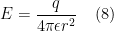
The normalized power gain pattern of an individual antenna element (half-wave dipole) is given by

\[G_{dipole}(\theta, \phi) = \frac{cos^2 (\frac{\pi}{2} cos \theta)}{sin^2 \theta} \quad \quad (11)\]

From the Figure 4 given in this post, the maximum value for the normalized power gain occurs at θ =90°=π/2 radians, i.e, along the xy plane.

\[G_{dipole}(\theta = \pi/2, \phi) = 1 \quad \quad (12)\]

The array factor for the arrangement in Figure 3, computed at θ =90°=π/2 radians is given by

\[A(\theta = \pi/2, \phi) = a_0 + a_1 e^{(j \frac{2 \pi}{\lambda} \; l\; cos \phi)} + a_2 e^{(j \;2\; \frac{2 \pi}{\lambda} \; l \; cos \phi)} \quad \quad (13)\]

The total normalized power gain, along the xy plane (θ =90°=π/2 radians), of the array of dipole antennas arranged as given in Figure 3, is given by

\[G_{total}\left( \theta = \pi/2, \phi \right) = \mid A(\theta = \pi/2, \phi)\mid ^2 G_{dipole}\left( \theta = \pi/2, \phi \right) \quad \quad (14)\]

Dropping the θ for convenience in representation

\[G_{total}\left( \phi \right) = \mid A(\phi)\mid ^2 G_{dipole}\left( \phi \right) \quad \quad (15)\]

Simulation

Figure 4 illustrates equation (15) – the effect of array factor on normalized power gain of an array of half-wave dipole antennas. The plot is generated for separation distance between antenna elements l=λ and the feed coefficients for the antenna elements a = [1, -1, 1].

Check out my Google colab for the python code. The results are given below.

Figure 4: Illustrating the effect of array pattern multiplication on normalized power gain of antenna array

References

[1] Orfanidis, S.J. (2013) Electromagnetic Waves and Antennas, Rutgers University. https://www.ece.rutgers.edu/~orfanidi/ewa/

[2] Constantine A. Balanis, Antenna Theory: Analysis and Design, ISBN: 978-1118642061, Wiley; 4th edition (February 1, 2016)

Far-field retarded potentials

Key focus: Far-field region is dominated by radiating terms of antenna fields, hence, knowing the far field retarded potentials is of interest.

Introduction

The fundamental premise of understanding antenna radiation is to understand how a radiation source influences the propagation of travelling electromagnetic waves. Propagation of travelling waves is best described by electric and magnetic potentials along the propagation path.

The concept of retarded potentials was introduced in this post.

The electromagnetic field travels at certain velocity and hence the potentials at the observation point (due to the changing charge at source) are experienced after a certain time delay. Such potentials are called retarded potentials.

The retarded potentials at a radial distance r from an antenna source fed with a single frequency sinusoidal waves, is shown to be

\[\begin{aligned} \Phi(r) &= \frac{1}{4 \pi \epsilon} \int_V \frac{\rho(z')e^{-j k R }}{R} d^3 z' \\ A(r) &= \frac{\mu}{4 \pi} \int_V \frac{J(z')e^{-j k R }}{R} d^3 z' \end{aligned} \quad \quad (1)\]

where, the quantity k = ω/c = 2 π/λ is called the free-space wavenumber. Also, ρ is the charge density, J is the current density, Φ is the electric potential and A is the magnetic potential that are functions of both radial distance.

Far-field region

Figure 1 illustrates the two scenarios: (a) the receiver is ‘nearer’ to the antenna source (b) the receiver is ‘far away’ from the antenna source.

Figure 1: Radiation fields when antenna and receiver are (a) near and (b) far away

Since the far-field region is dominated by radiating terms of the antenna fields, we are interested in knowing the retarded potentials in the far-field region. The far field region is shown to be

\[\frac{2 l^2}{ \lambda} < r < \infty \quad \quad (2)\]

where l is the length of the antenna element and λ is the wavelength of the signal from the antenna.

In the process of deriving the boundary between far-field and near-field, we used the following first order approximation for the radial distance R.

\[R = r – z' \; cos \theta= r – \hat{r} \cdot z' \quad \quad (3)\]

Far field retarded potential

Substituting this approximation in the numerator of equation (1) and replacing R by r in the denominator

\[\begin{aligned} \Phi(r) &= \frac{1}{4 \pi \epsilon} \int_V \frac{\rho(z')e^{-j k \left( r – \hat{r} \cdot z' \right) }}{r} d^3 z' \\ A(r) &= \frac{\mu}{4 \pi} \int_V \frac{J(z')e^{-j k \left( r – \hat{r} \cdot z'\right) }}{r} d^3 z' \end{aligned} \quad \quad (4)\]

The equation can be written as

\[\begin{aligned} \Phi(r) &= \frac{e^{-jkr}}{4 \pi \epsilon} \int_V \frac{\rho(z')e^{ j k \hat{r} \cdot z' }}{r} d^3 z' \\ A(r) &= \frac{\mu e^{-jkr}}{4 \pi} \int_V \frac{J(z')e^{j k \hat{r} \cdot z' }}{r} d^3 z' \end{aligned} \quad \quad (5)\]
Figure 2: Spherical coordinate system on a cartesian coordinate system

Antenna radiation patterns are generally visualized in a spherical coordinate system (Figure (2)). In a coordinate system, each unit vector can be expressed as the cross product of other two unit vectors. Hence,

\[\begin{aligned}\hat{r} &= \hat{\theta} \times \hat{\phi} \\ \hat{\theta} &= \hat{\phi} \times \hat{r} \\ \hat{\phi} &= \hat{r} \times \hat{\theta} \end{aligned} \quad \quad (6) \]

Therefore, the far-field retarded potentials in equation (5) can be written in terms of polar angle (θ) and azimuthal angle (ɸ)

\[\boxed{\begin{aligned} \Phi(r) &= \frac{e^{-jkr}}{4 \pi \epsilon r} \int_V \rho(z')e^{ j k \left( \hat{\theta} \times \hat{\phi} \right) \cdot z' } d^3 z' \\ A(r) &= \frac{\mu e^{-jkr}}{4 \pi r} \int_V J(z')e^{j k \left( \hat{\theta} \times \hat{\phi} \right) \cdot z' } d^3 z' \end{aligned}} \quad \quad (7)\]

We note that the term inside the integral is dependent on polar angle (θ) and azimuthal angle (ɸ). It determines the directional properties of the radiation. The term outside the integral is dependent on radial distance r. These terms can be expressed separately

\[\begin{aligned} \Phi(r) &= \frac{e^{-jkr}}{4 \pi \epsilon r} \mathbf{Q} \left(\theta, \phi \right) \\ A(r) &= \frac{\mu e^{-jkr}}{4 \pi r} \mathbf{F} \left(\theta, \phi \right) \end{aligned} \quad \quad (8)\]

The terms that determine the directional properties: Q(θ,ɸ) & F(θ,ɸ) are called charge form-factor and radiation vector respectively. The charge form-factor Q(θ,ɸ) and the radiation vector F(θ,ɸ) are three dimensional spatial Fourier transforms of charge density ρ(z’) and current density J(z) respectively.

\[\boxed{\begin{aligned} \mathbf{Q} \left(\theta, \phi \right) & = \int_V \rho(z')e^{ j k \left( \hat{\theta} \times \hat{\phi} \right) \cdot z' }d^3 z' \quad \quad \text{(charge form-factor)}\\ \mathbf{F} \left(\theta, \phi \right) &=\int_V J(z')e^{j k \left( \hat{\theta} \times \hat{\phi} \right) \cdot z' } d^3 z' \quad \quad \text{(radiation vector)} \end{aligned}}\quad \quad (9) \]

The charge-form factor and radiation vector can also be written in terms of direction of the unit vector of radial distance.

\[\boxed{\begin{aligned} \mathbf{Q} \left(\mathbf{k} \right) & = \int_V \rho(z')e^{ j \mathbf{k}\cdot z' }d^3 z' \quad \quad \text{(charge form-factor)} \\ \mathbf{F} \left(\mathbf{k}\right) &=\int_V J(z')e^{j \mathbf{k}\cdot z' } d^3 z' \quad \quad \text{(radiation vector)} \end{aligned}} \quad \quad \boxed{\mathbf{k} = k\hat{r}} \quad \quad (10) \]

Recap

We are in the process of building antenna models. In that journey, we started with the fundamental Maxwell’s equations in electromagnetism, then looked at retarded potentials that are solutions for Maxwell’s equations. Propagation of travelling waves is best described by retarded potentials along the propagation path. Then, the boundary between near-field and far-field regions was defined. Since most of the antenna radiation analysis are focused in the far-field regions, we looked at retarded potentials in the far-field region.

Rate this article: Note: There is a rating embedded within this post, please visit this post to rate it.

Books by the author


Wireless Communication Systems in Matlab
Second Edition(PDF)

(173 votes, average: 3.66 out of 5)

Checkout Added to cart

Digital Modulations using Python
(PDF ebook)

(127 votes, average: 3.58 out of 5)

Checkout Added to cart

Digital Modulations using Matlab
(PDF ebook)

(134 votes, average: 3.63 out of 5)

Checkout Added to cart
Hand-picked Best books on Communication Engineering
Best books on Signal Processing

Near-field – far-field : Where is the boundary ?

Antennas are radiation sources of finite physical dimension. To a distant observer, the radiation waves from the antenna source appears more like a spherical wave and the antenna appears to be a point source regardless of its true shape. The terms far-field and near-field are associated with such observations/antenna measurement. The terms imply that there must exist a boundary between the near field and far field.

Essentially, the near field and far field are regions around an antenna source. Though the boundary between these two regions are not fixed in space, the antenna measurements made in these regions differ significantly. One method of establishing the boundary between the near-field and far-field regions is to look at the acceptable level of phase error in the antenna measurements.

An antenna designer is interested in studying how the phase of the radiation waves launched from the antenna source is affected by the distance between the antenna source and the receiver (observation point). As the distance between the antenna and the receiver increases, there exists a phase difference between the measurements taken along the two lines shown. This phase difference contribute to antenna measurement errors, it also affects retarded potentials and radiation fields.

Near-field and far-field approximations

Figure 1 illustrates the two scenarios: (a) the receiver is ‘nearer’ to the antenna source (b) the receiver is ‘far away’ from the antenna source. The antenna is of standard dimension of length l. The figures show two rays – one from the origin to the observation point P (on the yz plane) and the other from the mid-point of distance z’=l/2 from the origin towards the observation point P.

In Figure(2)(b), the observation point P is at a distance that is very far from the antenna source element. The term ‘far’ implies that the distance r is much greater than the spatial extent of the current distribution of the antenna element, that is, r >> z’. Also, the two rays appear parallel to each other.

Figure 1: Radiation fields when antenna and receiver are (a) near and (b) far away

The essence of the following exercise is to determine the boundary between the ‘near’ and the ‘far’ field regions of the antenna. Once that boundary is established, we can determine whether far field approximation can be used on the antenna measurements or for the calculation of retarded potentials/fields produced by the antenna.

Let’s take a quick look at the retarded potentials derived for a single frequency wave emanating from the antenna source.

\[\begin{aligned} \Phi(r) &= \frac{1}{4 \pi \epsilon} \int_V \frac{\rho(z')e^{-j k R }}{R} d^3 z' \quad\quad (1) \\ A(r) &= \frac{\mu}{4 \pi} \int_V \frac{J(z')e^{-j k R }}{R} d^3 z' \quad\quad (2) \end{aligned}\]

We note that we cannot arbitrarily set R=r, because any small relative difference between R and r, will result in phase errors in the retarded potentials such that e-j k R ≠ e-j k r . Solving for the relationship between R and r is the crux of the radiation boundary problem.

From Figure (1)(a), applying law of cosines, the distance R can be written as

\[R = \sqrt{r^2 – 2 r z' cos \theta + z'^2} \quad \quad (3)\]

which can be expanded using the following Binomial series expansion,

\[ \begin{aligned}(x+y)^{n}&=\sum _{k=0}^{\infty }{n \choose k}x^{n-k}y^{k}\\&=x^{n}+nx^{n-1}y+{\frac {n(n-1)}{2!}}x^{n-2}y^{2}+{\frac {n(n-1)(n-2)}{3!}}x^{n-3}y^{3}+\cdots .\end{aligned}\]

Setting x = r2 and y= – 2 r z’ cos θ + z’ 2 , equation (3) can be expanded as

\[\begin{aligned} R & = r^{2(\frac{1}{2})}+\frac{1}{2}r^{2(\frac{1}{2}-1)} \left( -2 r z’ cos \theta + z’^2 \right )+\cdots .\\ & = r+ \frac{1}{2r} \left( -2 r z’ cos \theta + z’^2 \right ) – \frac{1}{8 r^3} \left(2 r z’ cos \theta \right )^2 + \cdots .\\ & = r – z’ cos \theta + \frac{z’^2}{2r} sin^2 \theta + \cdots . \end{aligned}\]

Neglecting the higher order terms,

\[\begin{aligned} R & \simeq r – z’ cos \theta + \frac{z’^2}{2r} sin^2 \theta \quad \quad (4) \end{aligned}\]

Truncation of equation (4) means we are dealing with the following maximum error in the antenna measurements:

\[\frac{z’^2}{2 r} sin^2 \theta = \frac{z’^2}{2 r} , \quad \quad \text{for } \theta=\frac{\pi}{2}\quad (5)\]

On the other hand, from Figure (1)(b), the distance \(R\) is given by

\[R = r – z’ cos \theta \quad \quad (6)\]

As r → ∞, equation (4) approaches exactly the parallel ray approximation given by equation (6). However, for finite values of r (due to the additional term z’ 2/2r sin2 θ and also the additional terms that were neglected) there exists an error between parallel ray approximation and the actual value of R computed using equation (4).

So the question is: What is the minimum distance over which the parallel ray approximation can be invoked ?

According to text books, for the maximum extent of the antenna (z’ = l/2), when the maximum phase difference is π/8, it produces acceptable errors in antenna measurements.

\[k \frac{z’^2}{2 r} \simeq \frac{\pi}{8} \quad \quad (7)\]

which gives

\[\boxed{r = \frac{2 l^2}{ \lambda}} \quad \quad (8)\]

In these equations, k = ω/c = 2 π/ λ is the free-space wavenumber.

Equation (8) defines the minimum distance (a.k.a the boundary between near and far field regions) over which the parallel ray approximation can be invoked. This minimum distance is called far-field distance – the boundary beyond which the far-field region starts. The quantity l is the maximum dimension of the antenna.

The far-field region, also known as Fraunhofer region, is dominated by radiating terms of the antenna fields. The far-field region is

\[\boxed{\frac{2 l^2}{ \lambda} < r < \infty }\quad \quad (9)\]
Figure 2: Far-field distance and far-field region

Rate this article: Note: There is a rating embedded within this post, please visit this post to rate it.

Books by the author


Wireless Communication Systems in Matlab
Second Edition(PDF)

Note: There is a rating embedded within this post, please visit this post to rate it.
Checkout Added to cart

Digital Modulations using Python
(PDF ebook)

Note: There is a rating embedded within this post, please visit this post to rate it.
Checkout Added to cart

Digital Modulations using Matlab
(PDF ebook)

Note: There is a rating embedded within this post, please visit this post to rate it.
Checkout Added to cart
Hand-picked Best books on Communication Engineering
Best books on Signal Processing

Retarded potentials

Key focus: Understand retarded potentials – the basic building block for understanding antenna array patterns. Retarded potentials are potentials at an observation point when the quantities at the source are non-static (varies in both space and time)

The static case : potentials

The fundamental premise of understanding antenna radiation is to understand how a radiation source influences the propagation of travelling electromagnetic waves. Propagation of travelling waves are best described by electric and magnetic potentials along the propagation path.

In the static case, the electric field E, charge density ρ, current density J and the electric potential Φ , magnetic field B and magnetic potential A are all constant in time. That is, they are functions of radial distance r in the spherical co-ordinate system, but not functions of time t . The solution for Maxwell’s equations (in the spherical co-ordinate system) take the following equivalent form in terms of electric and magnetic potentials:

\[\begin{aligned} \Phi(r) & = \frac{1}{4 \pi \epsilon} \int_V \frac{\rho(r')}{R} d^3 r' \quad \quad (1) \\ A(r) & = \frac{\mu}{4 \pi} \int_V \frac{J(r’)}{R} d^3 r’ \quad \quad (2) \end{aligned}\]
Figure 1: Potentials – solutions for Maxwell’s equations for static case

The quantity R is the distance between the source and the point at which the corresponding fields are observed and d3 r’ is the volume element at the source point.

The non-static case : retarded potentials

Since electromagnetic radiation are produced by time-varying electric charges, we are interested in describing the potentials at a given the observation point for this non-static situation. Obviously for the non-static case, the electric field E , charge density ρ , current density J and the electric potential Φ , magnetic field B and magnetic potential A are functions of both radial distance and time. The corresponding formulas for the potentials are

\[\begin{aligned} \Phi(r, t) & = \frac{1}{4 \pi \epsilon} \int_V \frac{\rho(r’, t – \frac{R}{c})}{R} d^3 r’ \quad \quad (3) \\ A(r, t) & = \frac{\mu}{4 \pi} \int_V \frac{J(r’, t – \frac{R}{c} )}{R} d^3 r’ \quad \quad (4) \end{aligned}\]

With c defined as the velocity of light, the factor t – R/c is the time delay between the emission of electromagnetic photon from the source and the time it gets observed by an observer. The electromagnetic field travels at certain velocity and hence the potentials at the observation point (due to the changing charge at source) are experienced after a certain time delay. Such potentials are called retarded potentials and the propagation delay t – R/c is called retarded time. Hence, we can say that the retarded potentials are related to electromagnetic fields of a current or charge distribution that vary in time.

Figure 2: Retarded potentials – solutions for Maxwell’s equations for non-static case

Sinusoidal time dependence of retarded potentials

In antenna theory, the antenna elements (source) are fed with sinusoidal waves. So, the next step is to express the retarded potentials at the observation point when all the quantities at source vary sinusoidally in time. Therefore, when the quantities are sinusoidal single-frequency waves, the shift property of Fourier transform can be applied.

\[\begin{aligned} \Phi(r, t) &= \Phi(r) e^{j \omega t} \\ \rho(r,t) &= \rho(r) e^{j \omega t} \\ A(r, t) &= A(r) e^{j \omega t} \\ J(r, t) &= J(r) e^{j \omega t} \end{aligned} \quad \quad (5)\]

Then, the retarded potential Φ(r,t) at the field observation point become,

\[\begin{aligned} \Phi(r, t) &= \frac{1}{4 \pi \epsilon} \int_V \frac{\rho(r', t – \frac{R}{c})}{R} d^3 r' \\ \Rightarrow \Phi(r) e^{j \omega t} & = \frac{1}{4 \pi \epsilon} \int_V \frac{\rho(r')e^{j \omega (t – \frac{R}{c})}}{R} d^3 r'\\ \Rightarrow \Phi(r) &= \frac{1}{4 \pi \epsilon} \int_V \frac{\rho(r')e^{-j \omega \frac{R}{c}}}{R} d^3 r'\\ \Rightarrow \Phi(r) &= \frac{1}{4 \pi \epsilon} \int_V \frac{\rho(r')e^{-j \frac{\omega}{c} R }}{R} d^3 r' \\ \Rightarrow \Phi(r) &= \frac{1}{4 \pi \epsilon} \int_V \frac{\rho(r')e^{-j k R }}{R} d^3 r' \end{aligned}\]

The retarded potential A(r,t) can be derived in a similar manner. Therefore, the retarded potentials (equations (3) and (4) ) for the single frequency sinusoidal wave is given by

\[\boxed{ \begin{aligned} \Phi(r) &= \frac{1}{4 \pi \epsilon} \int_V \frac{\rho(r')e^{-j k R }}{R} d^3 r' \\ A(r) &= \frac{\mu}{4 \pi} \int_V \frac{J(r')e^{-j k R }}{R} d^3 r' \end{aligned} }\]

In these equations, the quantity k = ω/c = 2 π/λ is called the free-space wavenumber.

Rate this article: Note: There is a rating embedded within this post, please visit this post to rate it.

Books by the author


Wireless Communication Systems in Matlab
Second Edition(PDF)

Note: There is a rating embedded within this post, please visit this post to rate it.
Checkout Added to cart

Digital Modulations using Python
(PDF ebook)

Note: There is a rating embedded within this post, please visit this post to rate it.
Checkout Added to cart

Digital Modulations using Matlab
(PDF ebook)

Note: There is a rating embedded within this post, please visit this post to rate it.
Checkout Added to cart
Hand-picked Best books on Communication Engineering
Best books on Signal Processing

From Maxwell’s equations to antenna array – part 1

Key focus: Briefly look at the building blocks of antenna array theory starting from the fundamental Maxwell’s equations in electromagnetism.

Maxwell’s equations

Maxwell’s equations are a collection of equations that describe the behavior of electromagnetic fields. The equations relate the electric fields () and magnetic fields () to their respective sources – charge density () and current density ( ).

Maxwell’s equations are available in two forms: differential form and integral form. The integral forms of Maxwell’s equations are helpful in their understanding the physical significance.

Maxwell’s equation (1):

The flux of the displacement electric field through a closed surface equals the total electric charge enclosed in the corresponding volume space .

This is also called Gauss law for electricity.

Consider a point charge +q in a three dimensional space. Assuming a symmetric field around the charge and at a distance r from the charge, the surface area of the sphere is .

Figure 1: Illustration of Coulomb’s law using Maxwell’s equation

Therefore, left side of the equation is simply equal to the surface area of the sphere multiplied by the magnitude of the electric displacement vector .

For the right hand side of the Maxwell’s equation (1), the integral of the charge density over a volume V is simply equal to the charge enclosed. Therefore,

The electric displacement field is a measure of electric field in the material after taking into account the effect of the material on the electric field. The electric field and the displacement field are related by the permittivity of the material as

Combining equations (5), (6) and (7), yields the magnitude of an electric field as derived from Coulomb’s law

Maxwell’s equation (2)

The flux of the magnetic field through a closed surface is zero. That is, the net of magnetic field that “flows into” and “flows out of” a closed surface is zero.

This implies that there are no source or sink for the magnetic flux lines, in other words – they are closed field lines with no beginning or end. This is also called Gauss law for magnetic field.

Figure 2: Gauss law for magnetic field

Maxwell’s equation (3)

The work done on an electric charge as it travels around a closed loop conductor is the electromotive force (emf). Therefore, the left side of the gives the emf induced in a circuit.

The right side of the equation is the rate of change of magnetic flux through the circuit.

Hence, the Maxwell’s third equation is actually the Faraday’s (and Len’s) law of magnetic induction

The electromotive force (emf) induced in a circuit is directly proportional to the rate of change of magnetic flux through the circuit.

Figure 3: Faraday’s law for magnetic induction

Maxwell’s equation (4)

The circulating magnetic field is denoted by the circulation of magnetizing field around a closed curved path : . The electric current is denoted by the flux of current density () through any surface spanning that curved path. The quantity denotes the rate of change of displacement current through any surface spanning that curved path.

According to Maxwell’s extension to the Ampere’s law , magnetic fields can be generated in two ways: with electric current and with changing electric flux. The equation states that the electric current or change in electric flux through a surface produces a circulating magnetic field around any path that bounds that surface.

Summary of Maxwell’s equations

The electric field leaving a volume space is proportional to the electric charge contained in the volume.

The net of magnetic field that “flows into” and “flows out of” a closed surface is zero. There is no concept called magnetic charge/magnetic monopole.

A changing magnetic flux through a circuit induces electromotive force in the circuit

Magnetic fields are produced by electric current as well as by changing electric flux.

Rate this article: Note: There is a rating embedded within this post, please visit this post to rate it.

References

[1] The Feynman lectures on physics – online edition ↗

Books by the author


Wireless Communication Systems in Matlab
Second Edition(PDF)

Note: There is a rating embedded within this post, please visit this post to rate it.
Checkout Added to cart

Digital Modulations using Python
(PDF ebook)

Note: There is a rating embedded within this post, please visit this post to rate it.
Checkout Added to cart

Digital Modulations using Matlab
(PDF ebook)

Note: There is a rating embedded within this post, please visit this post to rate it.
Checkout Added to cart
Hand-picked Best books on Communication Engineering
Best books on Signal Processing

Normalized power gain of dipole antennas

Key focus: Briefly look at linear antennas and various dipole antennas and plot the normalized power gain pattern in polar plot and three dimensional plot.

Linear antennas

Linear antennas are electrically thin antennas whose conductor diameter is very small compared to the wavelength of the radiation λ.

Viewed in a spherical coordinate system (Figure 1), for linear antenna, the antenna is oriented along the z-axis such that the radiation vector has only components along directions of the radial distance Fr and the polar angle Fθ. The radiation vector is determined by the current density J which is characterized by the current distribution I(z) [1].

Figure 1: Electrical and magnetic fields from a current source
Figure 2: Linear antenna element

Hertzian dipole (infinitesimally small dipole)

Hertzian dipole is the simplest configuration of a linear antenna used for study purposes. It is an infinitesimally small (typically [2]) antenna element that has the following current density distribution

\[I(z) = I \; L\; \delta(z)\]

The radiation vector Fz (θ) is given by [1]

\[F_z(\theta) = \int_{-L/2}^{L/2} I(z^{'}) e^{jk_z z^{'}} dz{'} = \int_{-L/2}^{L/2} I L \delta(z{'}) e^{jkz{'}cos \theta} dz{'} = IL\]

The normalized power gain of the Hertzian dipole is [2]

\[g(\theta) = C_0 sin^{2} \theta \]

where, C0 is a constant chosen to make maximum of g(θ) equal to unity and θ is the polar angle in the spherical coordinate system.

Center-fed dipole (standing wave antenna)

For the center-fed small dipole antenna, the current distribution is assumed to be a standing wave. Defining k = 2π/λ as the wave number and h = L/2 as the half-length of the antenna, the current distribution and the normalized power gain g(θ) are given by

\[I(z) = I \; sin \left[ k \left(L/2 – |z| \right) \right]\]
\[g(\theta) =C_n \left|\frac{cos (k h \; cos \theta) – cos( k h) }{sin \theta} \right| ^2\]

where, Cn is a constant chosen to make maximum of g(θ) equal to unity and θ is the polar angle in the spherical coordinate system.

Figure 3: Center-fed small dipole

For half-wave dipole, set L = λ/2 or kl = π. Therefore, the current distribution for half-wave dipole shrinks to

\[I(z) = I \; cos(kz)\]

The normalized power gain is

\[g(\theta) = C_2 \frac{cos^2 (\frac{\pi}{2} cos \theta)}{sin^2 \theta} \approx C_2 sin^3 \theta\]

Plotting the normalized power gain

Let’s plot the normalized power gain pattern of Hertzian & Half-wave dipole antennas in polar plot and three dimensional plot.

Check out my Google colab for the python code to plot the normalized power gain in polar plot as well as three dimensional plot. The results are given below.

Figure 4: Hertzian dipole – power gain pattern (polar plot)
Figure 5: Hertzian dipole – power gain pattern (3D plot)
Figure 6: Half-wave dipole – power gain pattern (polar plot)
Figure 7: Half-wave dipole power gain 3d plot (cartesian coordinates)
Figure 8: Normalized power gain pattern for dipole of length
Figure 9: Normalized power gain pattern for dipole of length (3D projection)

Rate this article: Note: There is a rating embedded within this post, please visit this post to rate it.

References

[1] Orfanidis, S.J. (2013) Electromagnetic Waves and Antennas, Rutgers University. https://www.ece.rutgers.edu/~orfanidi/ewa/

[2] Constantine A. Balanis, Antenna Theory: Analysis and Design, ISBN: 978-1118642061, Wiley; 4th edition (February 1, 2016)