Antennas are radiation sources of finite physical dimension. To a distant observer, the radiation waves from the antenna source appears more like a spherical wave and the antenna appears to be a point source regardless of its true shape. The terms far-field and near-field are associated with such observations/antenna measurement. The terms imply that there must exist a boundary between the near field and far field.
Essentially, the near field and far field are regions around an antenna source. Though the boundary between these two regions are not fixed in space, the antenna measurements made in these regions differ significantly. One method of establishing the boundary between the near-field and far-field regions is to look at the acceptable level of phase error in the antenna measurements.
An antenna designer is interested in studying how the phase of the radiation waves launched from the antenna source is affected by the distance between the antenna source and the receiver (observation point). As the distance between the antenna and the receiver increases, there exists a phase difference between the measurements taken along the two lines shown. This phase difference contribute to antenna measurement errors, it also affects retarded potentials and radiation fields.
Near-field and far-field approximations
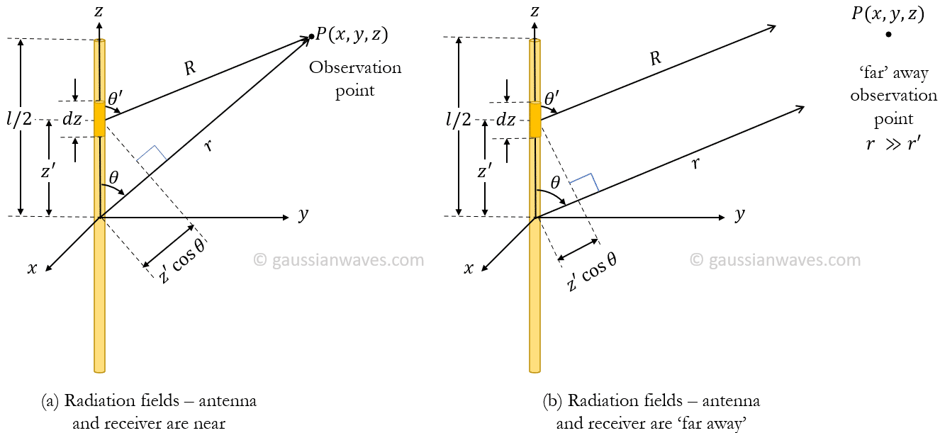
Figure 1 illustrates the two scenarios: (a) the receiver is ‘nearer’ to the antenna source (b) the receiver is ‘far away’ from the antenna source. The antenna is of standard dimension of length l. The figures show two rays – one from the origin to the observation point P (on the yz plane) and the other from the mid-point of distance z’=l/2 from the origin towards the observation point P.
In Figure(2)(b), the observation point P is at a distance that is very far from the antenna source element. The term ‘far’ implies that the distance r is much greater than the spatial extent of the current distribution of the antenna element, that is, r >> z’. Also, the two rays appear parallel to each other.
The essence of the following exercise is to determine the boundary between the ‘near’ and the ‘far’ field regions of the antenna. Once that boundary is established, we can determine whether far field approximation can be used on the antenna measurements or for the calculation of retarded potentials/fields produced by the antenna.
Let’s take a quick look at the retarded potentials derived for a single frequency wave emanating from the antenna source.
\[\begin{aligned} \Phi(r) &= \frac{1}{4 \pi \epsilon} \int_V \frac{\rho(z’)e^{-j k R }}{R} d^3 z’ \quad\quad (1) \\ A(r) &= \frac{\mu}{4 \pi} \int_V \frac{J(z’)e^{-j k R }}{R} d^3 z’ \quad\quad (2) \end{aligned}\]We note that we cannot arbitrarily set R=r, because any small relative difference between R and r, will result in phase errors in the retarded potentials such that e-j k R ≠ e-j k r . Solving for the relationship between R and r is the crux of the radiation boundary problem.
From Figure (1)(a), applying law of cosines, the distance R can be written as
\[R = \sqrt{r^2 – 2 r z’ cos \theta + z’^2} \quad \quad (3)\]which can be expanded using the following Binomial series expansion,
\[ \begin{aligned}(x+y)^{n}&=\sum _{k=0}^{\infty }{n \choose k}x^{n-k}y^{k}\\&=x^{n}+nx^{n-1}y+{\frac {n(n-1)}{2!}}x^{n-2}y^{2}+{\frac {n(n-1)(n-2)}{3!}}x^{n-3}y^{3}+\cdots .\end{aligned}\]Setting x = r2 and y= – 2 r z’ cos θ + z’ 2 , equation (3) can be expanded as
\[\begin{aligned} R & = r^{2(\frac{1}{2})}+\frac{1}{2}r^{2(\frac{1}{2}-1)} \left( -2 r z’ cos \theta + z’^2 \right )+\cdots .\\ & = r+ \frac{1}{2r} \left( -2 r z’ cos \theta + z’^2 \right ) – \frac{1}{8 r^3} \left(2 r z’ cos \theta \right )^2 + \cdots .\\ & = r – z’ cos \theta + \frac{z’^2}{2r} sin^2 \theta + \cdots . \end{aligned}\]Neglecting the higher order terms,
\[\begin{aligned} R & \simeq r – z’ cos \theta + \frac{z’^2}{2r} sin^2 \theta \quad \quad (4) \end{aligned}\]Truncation of equation (4) means we are dealing with the following maximum error in the antenna measurements:
\[\frac{z’^2}{2 r} sin^2 \theta = \frac{z’^2}{2 r} , \quad \quad \text{for } \theta=\frac{\pi}{2}\quad (5)\]On the other hand, from Figure (1)(b), the distance \(R\) is given by
\[R = r – z’ cos \theta \quad \quad (6)\]As r → ∞, equation (4) approaches exactly the parallel ray approximation given by equation (6). However, for finite values of r (due to the additional term z’ 2/2r sin2 θ and also the additional terms that were neglected) there exists an error between parallel ray approximation and the actual value of R computed using equation (4).
So the question is: What is the minimum distance over which the parallel ray approximation can be invoked ?
According to text books, for the maximum extent of the antenna (z’ = l/2), when the maximum phase difference is π/8, it produces acceptable errors in antenna measurements.
\[k \frac{z’^2}{2 r} \simeq \frac{\pi}{8} \quad \quad (7)\]which gives
\[\boxed{r = \frac{2 l^2}{ \lambda}} \quad \quad (8)\]In these equations, k = ω/c = 2 π/ λ is the free-space wavenumber.
Equation (8) defines the minimum distance (a.k.a the boundary between near and far field regions) over which the parallel ray approximation can be invoked. This minimum distance is called far-field distance – the boundary beyond which the far-field region starts. The quantity l is the maximum dimension of the antenna.
The far-field region, also known as Fraunhofer region, is dominated by radiating terms of the antenna fields. The far-field region is
\[\boxed{\frac{2 l^2}{ \lambda} < r < \infty }\quad \quad (9)\]
Rate this article: [ratings]
Books by the author
[table “23” not found /]