Frequency selective Archives

Model a Frequency Selective Multipath Fading channel

A brief intro to modeling a frequency selective fading channel using tapped delay line (TDL) filters. Rayleigh & Rician frequency-selective fading channel models explained.

Tapped delay line filters

Tapped-delay line filters (FIR filters) are best to simulate multiple echoes originating from same source. Hence they can be used to model multipath scenarios. Tapped-Delay-Line (TDL) filters with number taps can be used to simulate a multipath frequency selective fading channel. Frequency selective channels are characterized by time varying nature of the channel. For simulating a frequency selective channel, it is mandatory to have N > 1. In contrast, if N = 1, it simulates a zero-mean fading channel where all the multipath signals arrive at the receiver at the same time.

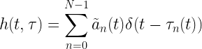
This article is part of the book Wireless Communication Systems in Matlab, ISBN: 978-1720114352 available in ebook (PDF) format (click here) and Paperback (hardcopy) format (click here).

Let be the associated path attenuation corresponding to the received power and propagation delay of the th path. In continuous time, the complex path attenuation is given by

The complex channel response is given by

In the equation above, the attenuation and path delay vary with time. This simulates a time-variant complex channel.

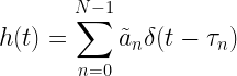
As a special case, in the absence any movements or other changes in the transmission channel, the channel can remain fairly time invariant (fixed channel with respect to instantaneous time ) even though the multipath is present. Thus the time-invariant complex channel becomes

Usually, the pair is described as a Power Delay Profile (PDP) plot. A sample power delay profile plot for a fixed, discrete, three ray model with its corresponding implementation using a tapped-delay line filter is shown in the following figure

Figure 1: 3-ray multipath time-invariant channel and its equivalent TDL implementation (path attenuations and
propagation delays are fixed)

Choose underlying distribution:

The next level of modeling involves, introduction of randomness in the above mentioned model there by rendering the channel response time variant. If the path attenuations are typically drawn from a complex Gaussian random variable, then at any given time , the absolute value of the impulse response is

● Rayleigh distributed – if the mean of the distribution
● Rician distributed – if the mean of the distribution

Respectively, these two scenarios model the presence or absence of a Line of Sight (LOS) path between the transmitter and the receiver. The first propagation delay has no effect on the model behavior and hence it can be removed.

Similarly, the propagation delays can also be randomized, resulting in a more realistic but extremely complex model to implement. Furthermore, the power-delay-profile specifications with arbitrary time delays, warrant non-uniformly spaced tapped-delay-line filters, that are not suitable for practical simulation. For ease of implementation, the given PDP model with arbitrary time delays can be converted to tractable uniformly spaced statistical model by a combination of interpolation/approximation/uniform-sampling of the given power-delay-profile.

Real-life modelling:

Usually continuous domain equations for modeling multipath are specified in standards like COST-207 model in GSM specification. Such continuous time power-delay-profile models can be simulated using discrete-time Tapped Delay Line (TDL) filter with number of taps with variable tap gains. Given the order , the problem boils down to determining the discrete tap spacing and the path gains , in such a way that the simulated channel closely follows the specified multipath PDP characteristics. A survey of method to find a solution for this problem can be found in [2].

Rate this article: Note: There is a rating embedded within this post, please visit this post to rate it.

References:

[1] Julius O. Smith III, Physical Audio Signal Processing, W3K Publishing, 2010, ISBN 978-0-9745607-2-4.↗
[2] M. Paetzold, A. Szczepanski, N. Youssef, Methods for Modeling of Specified and Measured Multipath Power-Delay Profiles, IEEE Trans. on Vehicular Techn., vol.51, no.5, pp.978-988, Sep.2002.↗

Topics in this chapter

Small-scale Models for Multipath Effects
● Introduction
● Statistical characteristics of multipath channels
□ Mutipath channel models
□ Scattering function
□ Power delay profile
□ Doppler power spectrum
□ Classification of small-scale fading
● Rayleigh and Rice processes
□ Probability density function of amplitude
□ Probability density function of frequency
● Modeling frequency flat channel
● Modeling frequency selective channel
□ Method of equal distances (MED) to model specified power delay profiles
□ Simulating a frequency selective channel using TDL model

Books by the author

Wireless Communication Systems in Matlab Second Edition(PDF) Note: There is a rating embedded within this post, please visit this post to rate it. Checkout Added to cart	Digital Modulations using Python (PDF ebook) Note: There is a rating embedded within this post, please visit this post to rate it. Checkout Added to cart	Digital Modulations using Matlab (PDF ebook) Note: There is a rating embedded within this post, please visit this post to rate it. Checkout Added to cart
Hand-picked Best books on Communication Engineering Best books on Signal Processing

Power Delay Profile

Power delay profile gives the signal power received on each multipath as a function of the propagation delays of the respective multipaths.

Power delay profile (PDP)

A multipath channel can be characterized in multiple ways for deterministic modeling and power delay profile (PDP) is one such measure. In a typical PDP plot, the signal power on each multipath is plotted against their respective propagation delays.

In a typical PDP plot, the signal power () of each multipath is plotted against their respective propagation delays (). A sample power delay profile plot, shown in Figure 1, indicates how a transmitted pulse gets received at the receiver with different signal strengths as it travels through a multipath channel with different propagation delays. PDP is usually supplied as a table of values, obtained from empirical data and it serves as a guidance to system design. Nevertheless, it is not an accurate representation of the real environment in which the mobile is destined to operate at.

Figure 1: A typical discrete power delay profile plot for a multipath channel with 3 paths

The PDP, when expressed as an intensity function , gives the signal intensity received over a multipath channel as a function of propagation delays. The PDP plots, like the one shown in Figure 1, can be obtained as the spatial average of the complex channel impulse response as

RMS delay spread and mean delay

The RMS delay spread and mean delay are two most important parameters that characterize a frequency selective channel. They are derived from power delay profile. The delay spread of a multipath channel at any time instant, is a measure of duration of time over which most of the symbol energy from the transmitter arrives the receiver.

This article is part of the book
● Wireless Communication Systems in Matlab (second edition), ISBN: 979-8648350779 available in ebook (PDF) format and Paperback (hardcopy) format.

In the wide-sense stationary uncorrelated scattering (WSSUS) channel models [1], the delays of received waves arriving at a receive antenna are treated as uncorrelated. Therefore, for the WSSUS model, the underlying complex process is assumed as zero-mean Gaussian random proces and hence the RMS value calculated from the normalized PDP corresponds to standard deviation of PDP distribution.

Figure 2: Relation between scattering function, power delay profile, Doppler power spectrum, spaced frequency
correlation function and spaced time correlation function

For continuous PDP (as in Figure 2), the RMS delay spread () can be calculated as

where, the mean delay is given by

For discrete PDP (as in Figure 1), the RMS delay spread () can be calculated as

where, is the power of the path, is the delay of the path and the mean delay is given by

Knowledge of the delay spread is essential in system design for determining the trade-off between the symbol rate of the system and the complexity of the equalizers at the receiver. The ratio of RMS delay spread () and symbol time duration () quantifies the strength of intersymbol interference (ISI). Typically, when the symbol time period is greater than 10 times the RMS delay spread, no ISI equalizer is needed in the receiver. The RMS delay spread obtained from the PDP must be compared with the symbol duration to arrive at this conclusion.

Frequency selective and non-selective channels

With the power delay profile, one can classify a multipath channel into frequency selective or frequency non-selective category. The derived parameter, namely, the maximum excess delay together with the symbol time of each transmitted symbol, can be used to classify the channel into frequency selective or non-selective channel.

PDP can be used to estimate the average power of a multipath channel, measured from the first signal that strikes the receiver to the last signal whose power level is above certain threshold. This threshold is chosen based on receiver design specification and is dependent on receiver sensitivity and noise floor at the receiver.

Maximum excess delay, also called maximum delay spread, denoted as (), is the relative time difference between the first signal component arriving at the receiver to the last component whose power level is above some threshold. Maximum delay spread () and the symbol time period () can be used to classify a channel into frequency selective or non-selective category. This classification can also be done using coherence bandwidth (a derived parameter from spaced frequency correlation function which in turn is the frequency domain representation of power delay profile).

Maximum excess delay is also an important parameter in mobile positioning algorithm. The accuracy of such algorithm depends on how well the maximum excess delay parameter conforms with measurement results from actual environment. When a mobile channel is modeled as a FIR filter (tapped delay line implementation), as in CODIT channel model [2], the number of taps of the FIR filter is determined by the product of maximum excess delay and the system sampling rate. The cyclic prefix in a OFDM system is typically determined by the maximum excess delay or by the RMS delay spread of that environment [3].

A channel is classified as frequency selective, if the maximum excess delay is greater than the symbol time period, i.e, . This introduces intersymbol interference into the signal that is being transmitted, thereby distorting it. This occurs since the signal components (whose powers are above either a threshold or the maximum excess delay), due to multipath, extend beyond the symbol time. Intersymbol interference can be mitigated at the receiver by an equalizer.

In a frequency selective channel, the channel output can be expressed as the convolution of input signal and the channel impulse response , plus some noise .

On the other hand, if the maximum excess delay is less than the symbol time period, i.e, , the channel is classified as frequency non-selective or zero-mean channel. Here, all the scattered signal components (whose powers are above either a specified threshold or the maximum excess delay) due to the multipath, arrive at the receiver within the symbol time. This will not introduce any ISI, but the received signal is distorted due to inherent channel effects like SNR condition. Equalizers in the receiver are not needed. A time varying non-frequency selective channel is obtained by assuming the impulse response . Thus the output of the channel can be expressed as

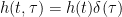
Therefore, for a frequency non-selective channel, the channel output can be expressed simply as product of time varying channel response and the input signal. If the channel impulse response is a deterministic constant, i.e, time invariant, then the non-frequency selective channel is expressed as follows by assuming

This is the simplest situation that can occur. In addition to that, if the noise in the above equation is white Gaussian noise, the channel is called additive white Gaussian noise (AWGN) channel.

Rate this article: Note: There is a rating embedded within this post, please visit this post to rate it.

References:

[1] P. A. Bello, Characterization of randomly time-variant linear channels, IEEE Trans. Comm. Syst., vol. 11, no. 4, pp. 360–393, Dec. 1963.↗
[2] Andermo, P.G and Larsson, G., Code division testbed, CODIT, Universal Personal communications, 1993. Personal Communications, Gateway to the 21st Century. Conference Record., 2nd International Conference on , vol.1, no., pp.397,401 vol.1, 12-15 Oct 1993.↗
[3] Huseyin Arslan, Cognitive Radio, Software Deﬁned Radio, and Adaptive Wireless Systems, pp. 238, 2007, Dordrecht, Netherlands, Springer.↗

Topics in this chapter

Books by the author

Wireless Communication Systems in Matlab Second Edition(PDF) Note: There is a rating embedded within this post, please visit this post to rate it. Checkout Added to cart	Digital Modulations using Python (PDF ebook) Note: There is a rating embedded within this post, please visit this post to rate it. Checkout Added to cart	Digital Modulations using Matlab (PDF ebook) Note: There is a rating embedded within this post, please visit this post to rate it. Checkout Added to cart
Hand-picked Best books on Communication Engineering Best books on Signal Processing

Fading channel – complex baseband equivalent models

Keyfocus: Fading channel models for simulation. Learn how fading channels can be modeled as FIR filters for simplified modulation & detection. Rayleigh/Rician fading.

Introduction

A fading channel is a wireless communication channel in which the quality of the signal fluctuates over time due to changes in the transmission environment. These changes can be caused by different factors such as distance, obstacles, and interference, resulting in attenuation and phase shifting. The signal fluctuations can cause errors or loss of information during transmission.

Fading channels are categorized into slow fading and fast fading depending on the rate of channel variation. Slow fading occurs over long periods, while fast fading happens rapidly over short periods, typically due to multipath interference.

To overcome the negative effects of fading, various techniques are used, including diversity techniques, equalization, and channel coding.

Fading channel in frequency domain

With respect to the frequency domain characteristics, the fading channels can be classified into frequency selective and frequency-flat fading.

A frequency flat fading channel is a wireless communication channel where the attenuation and phase shift of the signal are constant across the entire frequency band. This means that the signal experiences the same amount of fading at all frequencies, and there is no frequency-dependent distortion of the signal.

In contrast, a frequency selective fading channel is a wireless communication channel where the attenuation and phase shift of the signal vary with frequency. This means that the signal experiences different levels of fading at different frequencies, resulting in a frequency-dependent distortion of the signal.

Frequency selective fading can occur due to various factors such as multipath interference and the presence of objects that scatter or absorb certain frequencies more than others. To mitigate the effects of frequency selective fading, various techniques can be used, such as equalization and frequency hopping.

The channel fading can be modeled with different statistics like Rayleigh, Rician, Nakagami fading. The fading channel models, in this section, are utilized for obtaining the simulated performance of various modulations over Rayleigh flat fading and Rician flat fading channels. Modeling of frequency selective fading channel is discussed in this article.

Linear time invariant channel model and FIR filters

The most significant feature of a real world channel is that the channel does not immediately respond to the input. Physically, this indicates some sort of inertia built into the channel/medium, that takes some time to respond. As a consequence, it may introduce distortion effects like inter-symbol interference (ISI) at the channel output. Such effects are best studied with the linear time invariant (LTI) channel model, given in Figure 1.

*Figure 1: Complex baseband equivalent LTI channel model*

In this model, the channel response to any input depends only on the channel impulse response(CIR) function of the channel. The CIR is usually defined for finite length \(L\) as \(\mathbf{h}=[h_0,h_1,h_2, \cdots,h_{L-1}]\) where \(h_0\) is the CIR at symbol sampling instant \(0T_{sym}\) and \(h_{L-1}\) is the CIR at symbol sampling instant \((L-1)T_{sym}\). Such a channel can be modeled as a tapped delay line (TDL) filter, otherwise called finite impulse response (FIR) filter. Here, we only consider the CIR at symbol sampling instances. It is well known that the output of such a channel (\(\mathbf{r}\)) is given as the linear convolution of the input symbols (\(\mathbf{s}\)) and the CIR (\(\mathbf{h}\)) at symbol sampling instances. In addition, channel noise in the form of AWGN can also be included the model. Therefore, the resulting vector of from the entire channel model is given as

\[\mathbf{r} = \mathbf{h} \ast \mathbf{s} +\mathbf{n} \quad\quad (1) \]

This article is part of the following books
● Digital Modulations using Matlab : Build Simulation Models from Scratch, ISBN: 978-1521493885
● Digital Modulations using Python ISBN: 978-1712321638
● Wireless communication systems in Matlab ISBN: 979-8648350779
All books available in ebook (PDF) and Paperback formats

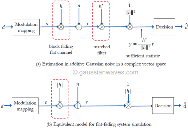
Simulation model for detection in flat fading channel

A flat-fading (also called as frequency-non-selective) channel is modeled with a single tap (\(L=1\)) FIR filter with the tap weights drawn from distributions like Rayleigh, Rician or Nakagami distributions. We will assume block fading, which implies that the fading process is approximately constant for a given transmission interval. For block fading, the random tap coefficient \(h=h[0]\) is a complex random variable (not random processes) and for each channel realization, a new set of complex random values are drawn from Rayleigh or Rician or Nakagami fading according to the type of fading desired.

*Figure 2: LTI channel viewed as tapped delay line filter*

Simulation models for modulation and detection over a fading channel is shown in Figure 2. For a flat fading channel, the output of the channel can be expressed simply as the product of time varying channel response and the input signal. Thus, equation (1) can be simplified (refer this article for derivation) as follows for the flat fading channel.

\[\mathbf{r} = h\mathbf{s} + \mathbf{n} \quad\quad (2) \]

Since the channel and noise are modeled as a complex vectors, the detection of \(\mathbf{s}\) from the received signal is an estimation problem in the complex vector space.

*Figure 3: Simulation model for modulation and detection over flat fading channel*

Assuming perfect channel knowledge at the receiver and coherent detection, the receiver shown in Figure 3(a) performs matched filtering. The impulse response of the matched filter is matched to the impulse response of the flat-fading channel as \( h^{\ast}\). The output of the matched filter is scaled down by a factor of \(||h||^2\) which is the total-energy contained in the impulse response of the flat-fading channel. The resulting decision vector \(\mathbf{y}\) serves as the sufficient statistic for the estimation of \(\mathbf{s}\) from the received signal \(\mathbf{r}\) (refer equation A.77 in reference [1])

\[\tilde{\mathbf{y}} = \frac{h^{\ast}}{||h||^2} \mathbf{r} = \frac{h^{\ast}}{||h||^2} h\mathbf{s} + \frac{h^{\ast}}{||h||^2} \mathbf{n} = \mathbf{s} + \tilde{\mathbf{w}} \quad\quad (3) \]

Since the absolute value \(|h|\) and the Eucliden norm \(||h||\) are related as \(|h|^2= \left\lVert h\right\rVert = hh^{\ast}\), the model can be simplified further as given in Figure 3(b).

To simulate flat fading, the values for the fading variable \(h\) are drawn from complex normal distribution

\[h= X + jY \quad\quad (4) \]

where, \(X,Y\) are statistically independent real valued normal random variables.

● If \(E[h]=0\), then \(|h|\) is Rayleigh distributed, resulting in a Rayleigh flat fading channel
● If \(E[h] \neq 0\), then \(|h|\) is Rician distributed, resulting in a Rician flat fading channel with the factor \(K=[E[h]]^2/\sigma^2_h\)

References

[1] D. Tse and P. Viswanath, Fundamentals of Wireless Communication, Cambridge University Press, 2005.↗

Books by the author

Wireless Communication Systems in Matlab Second Edition(PDF) Note: There is a rating embedded within this post, please visit this post to rate it. Checkout Added to cart	Digital Modulations using Python (PDF ebook) Note: There is a rating embedded within this post, please visit this post to rate it. Checkout Added to cart	Digital Modulations using Matlab (PDF ebook) Note: There is a rating embedded within this post, please visit this post to rate it. Checkout Added to cart
Hand-picked Best books on Communication Engineering Best books on Signal Processing

Cookie	Duration	Description
cookielawinfo-checbox-analytics	11 months	This cookie is set by GDPR Cookie Consent plugin. The cookie is used to store the user consent for the cookies in the category "Analytics".
cookielawinfo-checbox-analytics	11 months	This cookie is set by GDPR Cookie Consent plugin. The cookie is used to store the user consent for the cookies in the category "Analytics".
cookielawinfo-checbox-functional	11 months	The cookie is set by GDPR cookie consent to record the user consent for the cookies in the category "Functional".
cookielawinfo-checbox-functional	11 months	The cookie is set by GDPR cookie consent to record the user consent for the cookies in the category "Functional".
cookielawinfo-checbox-others	11 months	This cookie is set by GDPR Cookie Consent plugin. The cookie is used to store the user consent for the cookies in the category "Other.
cookielawinfo-checbox-others	11 months	This cookie is set by GDPR Cookie Consent plugin. The cookie is used to store the user consent for the cookies in the category "Other.
cookielawinfo-checkbox-necessary	11 months	This cookie is set by GDPR Cookie Consent plugin. The cookies is used to store the user consent for the cookies in the category "Necessary".
cookielawinfo-checkbox-performance	11 months	This cookie is set by GDPR Cookie Consent plugin. The cookie is used to store the user consent for the cookies in the category "Performance".
viewed_cookie_policy	11 months	The cookie is set by the GDPR Cookie Consent plugin and is used to store whether or not user has consented to the use of cookies. It does not store any personal data.