Generate color noise using Auto-Regressive (AR) model

Key focus: Learn how to generate color noise using auto regressive (AR) model. Apply Yule Walker equations for generating power law noises: pink noise, Brownian noise.

Auto-Regressive (AR) model

An uncorrelated Gaussian random sequence can be transformed into a correlated Gaussian random sequence using an AR time-series model. If a time series random sequence is assumed to be following an auto-regressive model of form,

where is the uncorrelated Gaussian sequence of zero mean and variance , the natural tendency is to estimate the model parameters . Least Squares method can be applied here to find the model parameters, but the computations become cumbersome as the order increases. Fortunately, the AR model coefficients can be solved for using Yule Walker equations.

Yule Walker equations relate auto-regressive model parameters to the auto-correlation of random process . Finding the model parameters using Yule-Walker equations, is a two step process:

1. Given , estimate auto-correlation of the process . If is already specified as a function, utilize it as it is (see auto-correlation equations for Jakes spectrum or Doppler spectrum in section 11.3.2 in the book).

2. Solve Yule Walker equations to find the model parameters and the noise sigma .

Yule-Walker equations

Yule-Walker equations can be compactly written as

Equation (2) Yule Walker equation

Written in matrix form, the Yule-Walker equations that comprises of a set of linear equations and unknown parameters.

Representing equation (3) in a compact form,

The AR model parameters can be found by solving

After solving for the model parameters , the noise variance can be found by applying the estimated values of in equation (2) by setting . The aryule command (in Matlab and Python’s spectrum package) efficiently solves the Yule-Walker equations using Levinson Algorithm [1][2]. Once the model parameters are obtained, the AR model can be implemented as an \emph{infinte impulse response (IIR)} filter of form

Example: power law noise generation

The power law in the power spectrum characterizes the fluctuating observables in many natural systems. Many natural systems exhibit some noise which is a stochastic process with a power spectral density having a power exponent that can take values . Simply put, noise is a colored noise with a power spectral density of over its entire frequency range.

The noise can be classified into different types based on the value of .

Violet noise – = -2, the power spectral density is proportional to .
Blue noise – = -1, the power spectral density is proportional to .
White noise – = 0, the power spectral density is flat across the whole spectrum.
Pink noise – = 1, the power spectral density is proportional to , i.e, it decreases by per octave with increase in frequency.
Brownian noise – = 2, the power spectral density is proportional to , therefore it decreases by per octave with increase in frequency.

The power law noise can be generated by sequencing a zero-mean white noise through an auto-regressive (AR) filter of order :

where, is a zero-mean white noise process. Referring the AR generation method described in [3], the coefficients of the AR filter can be generated as

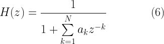
which can be implemented as an infinite impulse response (IIR) filter using the filter transfer function described in equation (6).

The following script implements this method and the sample results are plotted in the next Figure.

Refer the book for the Matlab code

Figure 1: Simulated color noise samples and their PSD estimates: pink noise (α =1) and Brown noise (α =2)

Rate this article: Note: There is a rating embedded within this post, please visit this post to rate it.

References

[1] Gene H. Golub, Charles F. Van Loan, Matrix Computations, ISBN-9780801854149, Johns Hopkins University Press, 1996, p. 143.↗
[2] J. Durbin, The fitting of time series in models, Review of the International Statistical Institute, 28:233-243, 1960.↗
[3] Kasdin, N.J. Discrete Simulation of Colored Noise and Stochastic Processes and Power Law Noise Generation, Proceedings of the IEEE, Vol. 83, No. 5, 1995, pp. 802-827.↗

Rate this article: Note: There is a rating embedded within this post, please visit this post to rate it.

Books by the author


Wireless Communication Systems in Matlab
Second Edition(PDF)

Note: There is a rating embedded within this post, please visit this post to rate it.
Checkout Added to cart

Digital Modulations using Python
(PDF ebook)

Note: There is a rating embedded within this post, please visit this post to rate it.
Checkout Added to cart

Digital Modulations using Matlab
(PDF ebook)

Note: There is a rating embedded within this post, please visit this post to rate it.
Checkout Added to cart
Hand-picked Best books on Communication Engineering
Best books on Signal Processing

Topics in this chapter

Random Variables - Simulating Probabilistic Systems
● Introduction
Plotting the estimated PDF
● Univariate random variables
 □ Uniform random variable
 □ Bernoulli random variable
 □ Binomial random variable
 □ Exponential random variable
 □ Poisson process
 □ Gaussian random variable
 □ Chi-squared random variable
 □ Non-central Chi-Squared random variable
 □ Chi distributed random variable
 □ Rayleigh random variable
 □ Ricean random variable
 □ Nakagami-m distributed random variable
Central limit theorem - a demonstration
● Generating correlated random variables
 □ Generating two sequences of correlated random variables
 □ Generating multiple sequences of correlated random variables using Cholesky decomposition
Generating correlated Gaussian sequences
 □ Spectral factorization method
 □ Auto-Regressive (AR) model

Generating colored noise with Jakes PSD: Spectral factorization

The aim of this article is to demonstrate the application of spectral factorization method in generating colored noise having Jakes power spectral density. Before continuing, I urge the reader to go through this post: Introduction to generating correlated Gaussian sequences.

This article is part of the book
Wireless Communication Systems in Matlab (second edition), ISBN: 979-8648350779 available in ebook (PDF) format and Paperback (hardcopy) format.

In spectral factorization method, a filter is designed using the desired frequency domain characteristics (like PSD) to transform an uncorrelated Gaussian sequence into a correlated sequence . In the model shown in Figure 1, the input to the LTI system is a white noise whose amplitude follows Gaussian distribution with zero mean and variance and the power spectral density (PSD) of the white noise is a constant across all frequencies.

The white noise sequence drives the LTI system with frequency response producing the signal of interest . The PSD of the output process is therefore

Figure 1: Relationship among various power spectral densities in a filtering process

If the desired power spectral density of the colored noise sequence is given, assuming , the impulse response of the LTI filter can be found by taking the inverse Fourier transform of the frequency response

Once, the impulse response of the filter is obtained, the colored noise sequence can be produced by driving the filter with a zero-mean white noise sequence of unit variance.

Example: Generating colored noise with Jakes PSD

For example, we wish to generate a Gaussian noise sequence whose power spectral density follows the normalized Jakes power spectral density (see section 11.3.2 in the book) given by

Applying spectral factorization method, the frequency response of the desired filter is

The impulse response of the filter is [1]

where, is the fractional Bessel function of the first kind, is the sampling interval for implementing the digital filter and is a constant. The impulse response of the filter can be normalized by dividing by .

The filter can be implemented as a finite impulse response (FIR) filter structure. However, the FIR implementation requires that the impulse response be truncated to a reasonable length. Such truncation leads to ringing effects due to Gibbs phenomenon. To avoid distortions due to truncation, the filter impulse response is usually windowed using a window function such as Hamming window.

where, the Hamming window is defined as

The function given in the book in section 2.6.1 implements a windowed Jakes filter using the aforementioned equations. The impulse response and the spectral characteristics of the filter are plotted in Figure 2.

Figure 2: Impulse response & spectrum of windowed Jakes filter ( fmax = 10Hz; Ts = 0:01s; N = 512)

A white noise can be transformed into colored noise sequence with Jakes PSD, by processing the white noise through the implemented filter. The script (given in the book in section 2.6.1)  illustrates this concept by transforming a white noise sequence into a colored noise sequence. The simulated noise samples and its PSD are plotted in Figure 3.

Rate this article: Note: There is a rating embedded within this post, please visit this post to rate it.

Reference

[1] Jeruchim et., al, Simulation of communication systems – modeling, methodology, and techniques, second edition, Kluwer academic publishers, 2002, ISBN: 0306462672.↗

Books by the author


Wireless Communication Systems in Matlab
Second Edition(PDF)

Note: There is a rating embedded within this post, please visit this post to rate it.
Checkout Added to cart

Digital Modulations using Python
(PDF ebook)

Note: There is a rating embedded within this post, please visit this post to rate it.
Checkout Added to cart

Digital Modulations using Matlab
(PDF ebook)

Note: There is a rating embedded within this post, please visit this post to rate it.
Checkout Added to cart
Hand-picked Best books on Communication Engineering
Best books on Signal Processing

Topics in this chapter

Random Variables - Simulating Probabilistic Systems
● Introduction
Plotting the estimated PDF
● Univariate random variables
 □ Uniform random variable
 □ Bernoulli random variable
 □ Binomial random variable
 □ Exponential random variable
 □ Poisson process
 □ Gaussian random variable
 □ Chi-squared random variable
 □ Non-central Chi-Squared random variable
 □ Chi distributed random variable
 □ Rayleigh random variable
 □ Ricean random variable
 □ Nakagami-m distributed random variable
Central limit theorem - a demonstration
● Generating correlated random variables
 □ Generating two sequences of correlated random variables
 □ Generating multiple sequences of correlated random variables using Cholesky decomposition
Generating correlated Gaussian sequences
 □ Spectral factorization method
 □ Auto-Regressive (AR) model

Generate correlated Gaussian sequence (colored noise)

Key focus: Colored noise sequence (a.k.a correlated Gaussian sequence), is a non-white random sequence, with non-constant power spectral density across frequencies.

Introduction

Speaking of Gaussian random sequences such as Gaussian noise, we generally think that the power spectral density (PSD) of such Gaussian sequences is flat.We should understand that the PSD of a Gausssian sequence need not be flat. This bring out the difference between white and colored random sequences, as captured in Figure 1.

A white noise sequence is defined as any random sequence whose PSD is constant across all frequencies. Gaussian white noise is a Gaussian random sequence, whose amplitude is gaussian distributed and its PSD is a constant. Viewed in another way, a constant PSD in frequency domain implies that the average auto-correlation function in time-domain is an impulse function (Dirac-delta function). That is, the amplitude of noise at any given time instant is correlated only with itself. Therefore, such sequences are also referred as uncorrelated random sequences. White Gaussian noise processes are completely characterized by its mean and variance.

This article is part of the book
Wireless Communication Systems in Matlab (second edition), ISBN: 979-8648350779 available in ebook (PDF) format and Paperback (hardcopy) format.

Figure 1: Power spectral densities of white noise and colored noise

A colored noise sequence is simply a non-white random sequence, whose PSD varies with frequency. For a colored noise, the amplitude of noise at any given time instant is correlated with the amplitude of noise occurring at other instants of time. Hence, colored noise sequences will have an auto-correlation function other than the impulse function. Such sequences are also referred as correlated random sequences. Colored
Gaussian noise processes are completely characterized by its mean and the shaped of power spectral density (or the shape of auto-correlation function).

In mobile channel model simulations, it is often required to generate correlated Gaussian random sequences with specified mean and power spectral density (like Jakes PSD or Gaussian PSD given in section 11.3.2 in the book). An uncorrelated Gaussian sequence can be transformed into a correlated sequence through filtering or linear transformation, that preserves the Gaussian distribution property of amplitudes, but alters only the correlation property (equivalently the power spectral density). We shall see two methods to generate colored Gaussian noise for given mean and PSD shape

Spectral factorization method
Auto-regressive (AR) model

Motivation

Let’s say we observe a real world signal that has an arbitrary spectrum . We would like to describe the long sequence of using very few parameters, as in applications like linear predictive coding (LPC). The modeling approach, described here, tries to answer the following two questions:

• Is it possible to model the first order (mean/variance) and second order (correlations, spectrum) statistics of the signal just by shaping a white noise spectrum using a transfer function ? (see Figure 1).
• Does this produce the same statistics (spectrum, correlations, mean and variance) for a white noise input ?

If the answer is yes to the above two questions, we can simply set the modeled parameters of the system and excite the system with white noise, to produce the desired real world signal. This reduces the amount to data we wish to transmit in a communication system application. This approach can be used to transform an uncorrelated white Gaussian noise sequence to a colored Gaussian noise sequence with desired spectral properties.

Linear time invariant (LTI) system model

In the given model, the random signal is observed. Given the observed signal , the goal here is to find a model that best describes the spectral properties of under the following assumptions
• The sequence is WSS (wide sense stationary) and ergodic.
• The input sequence to the LTI system is white noise, whose amplitudes follow Gaussian distribution with zero-mean and variance with flat the power spectral density.
• The LTI system is BIBO (bounded input bounded output) stable.

Read the continuation of this post : Spectral factorization method

Rate this article: Note: There is a rating embedded within this post, please visit this post to rate it.

Reference

[1] Jeruchim et., al, Simulation of communication systems – modeling, methodology, and techniques, second edition, Kluwer academic publishers, 2002, ISBN: 0306462672.↗

Books by the author


Wireless Communication Systems in Matlab
Second Edition(PDF)

Note: There is a rating embedded within this post, please visit this post to rate it.
Checkout Added to cart

Digital Modulations using Python
(PDF ebook)

Note: There is a rating embedded within this post, please visit this post to rate it.
Checkout Added to cart

Digital Modulations using Matlab
(PDF ebook)

Note: There is a rating embedded within this post, please visit this post to rate it.
Checkout Added to cart
Hand-picked Best books on Communication Engineering
Best books on Signal Processing

Topics in this chapter

Random Variables - Simulating Probabilistic Systems
● Introduction
Plotting the estimated PDF
● Univariate random variables
 □ Uniform random variable
 □ Bernoulli random variable
 □ Binomial random variable
 □ Exponential random variable
 □ Poisson process
 □ Gaussian random variable
 □ Chi-squared random variable
 □ Non-central Chi-Squared random variable
 □ Chi distributed random variable
 □ Rayleigh random variable
 □ Ricean random variable
 □ Nakagami-m distributed random variable
Central limit theorem - a demonstration
● Generating correlated random variables
 □ Generating two sequences of correlated random variables
 □ Generating multiple sequences of correlated random variables using Cholesky decomposition
Generating correlated Gaussian sequences
 □ Spectral factorization method
 □ Auto-Regressive (AR) model