Maximum Likelihood Estimation (MLE) : Understand with example

Key focus: Understand maximum likelihood estimation (MLE) using hands-on example. Know the importance of log likelihood function and its use in estimation problems.

Likelihood Function:

Suppose X=(x₁,x₂,…, x_N) are the samples taken from a random distribution whose PDF is parameterized by the parameter θ. The likelihood function is given by

Here f_N(x_N;θ) is the PDF of the underlying distribution.

The above equation differs significantly from the joint probability calculation that in joint probability calculation, θ is considered a random variable. In the above equation, the parameter θ is the parameter to be estimated.

Example:

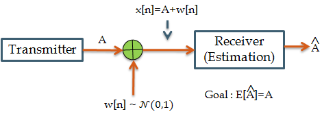
Consider the DC estimation problem presented in the previous article where a transmitter transmits continuous stream of data samples representing a constant value – A. The data samples sent via a communication channel gets added with White Gaussian Noise – w[n] (with μ=0 and σ²=1 ). The receiver receives the samples and its goal is to estimate the actual DC component – A in the presence of noise.

Likelihood as an Estimation Metric:

Let’s use the likelihood function as estimation metric. The estimation of A depends on the PDF of the underlying noise-w[n]. The estimation accuracy depends on the variance of the noise. More the variance less is the accuracy of estimation and vice versa.

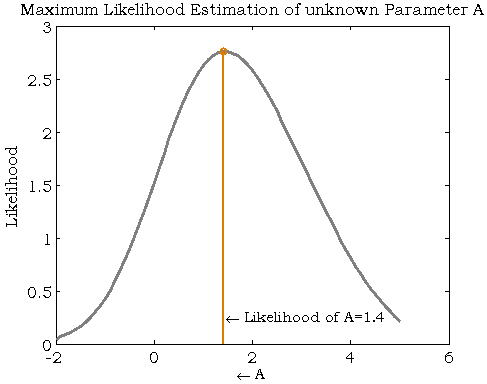
Let’s fix A=1.3 and generate 10 samples from the above model (Use the Matlab script given below to test this. You may get different set of numbers). Now we pretend that we do not know anything about the model and all we want to do is to estimate the DC component (Parameter to be estimated θ=A) from the observed samples:

Assuming a variance of 1 for the underlying PDF, we will try a range of values for A from -2.0 to +1.5 in steps of 0.1 and calculate the likelihood function for each value of A.

Matlab script:

% Demonstration of Maximum Likelihood Estimation in Matlab
%   Author: Mathuranathan (https://www.gaussianwaves.com)
%   License : creative commons : Attribution-NonCommercial-ShareAlike 3.0 Unported

A=1.3;
N=10; %Number of Samples to collect
x=A+randn(1,N);

s=1; %Assume standard deviation s=1

rangeA=-2:0.1:5; %Range of values of estimation parameter to test
L=zeros(1,length(rangeA)); %Place holder for likelihoods

for i=1:length(rangeA)
    %Calculate Likelihoods for each parameter value in the range
    L(i) = exp(-sum((x-rangeA(i)).^2)/(2*s^2));  %Neglect the constant term (1/(sqrt(2*pi)*sigma))^N as it will pull %down the likelihood value to zero for increasing value of N
end

[maxL,index]=max(L); %Select the parameter value with Maximum Likelihood
display('Maximum Likelihood of A');
display(rangeA(index));

%Plotting Commands
plot(rangeA,L);hold on;
stem(rangeA(index),L(index),'r'); %Point the Maximum Likelihood Estimate
displayText=['\leftarrow Likelihood of A=' num2str(rangeA(index))];
title('Maximum Likelihood Estimation of unknown Parameter A');
xlabel('\leftarrow A');
ylabel('Likelihood');
text(rangeA(index),L(index)/3,displayText,'HorizontalAlignment','left');

figure(2);
plot(rangeA,log(L));hold on;
YL = ylim;YMIN = YL(1);
plot([rangeA(index) rangeA(index)],[YMIN log(L(index))] ,'r'); %Point the Maximum Likelihood Estimate
title('Log Likelihood Function');
xlabel('\leftarrow A');
ylabel('Log Likelihood');
text([rangeA(index)],YMIN/2,displayText,'HorizontalAlignment','left');

Simulation Result:

For the above mentioned 10 samples of observation, the likelihood function over the range (-2:0.1:1.5) of DC component values is plotted below. The maximum likelihood value happens at A=1.4 as shown in the figure. The estimated value of A is 1.4 since the maximum value of likelihood occurs there.

This estimation technique based on maximum likelihood of a parameter is called Maximum Likelihood Estimation (MLE). The estimation accuracy will increase if the number of samples for observation is increased. Try the simulation with the number of samples N set to 5000 or 10000 and observe the estimated value of A for each run.

Log Likelihood Function:

It is often useful to calculate the log likelihood function as it reduces the above mentioned equation to series of additions instead of multiplication of several terms. This is particularly useful when implementing the likelihood metric in digital signal processors. The log likelihood is simply calculated by taking the logarithm of the above mentioned equation. The decision is again based on the maximum likelihood criterion.

$latex \begin{aligned} ln \left[L(\theta;X)\right ] &= \prod_{i=1}^{N} ln \left[f_i(x_i;\theta)\right ] \\
&= ln\left[f_1(x_1;\theta) \right ]+ln\left[f_2(x_2;\theta) \right ] + \cdots+ ln\left[f_N(x_N;\theta) \right ]
\end{aligned} &s=1$

The corresponding plot is given below

Advantages of Maximum Likelihood Estimation:

* Asymptotically Efficient – meaning that the estimate gets better with more samples
* Asymptotically unbiased
* Asymptotically consistent
* Easier to compute
* Estimation without any prior information
* The estimates closely agree with the data

Disadvantages of Maximum Likelihood Estimation:

* Since the estimates closely agree with data, it will give noisy estimates for data mixed with noise.
* It does not utilize any prior information for the estimation. But in real world scenario, we always have some prior information about the parameter to be estimated. We should always use it to our advantage despite it introducing bias in the estimates.

Rate this article: (10 votes, average: 4.40 out of 5)

For further reading

[1] Steven M. Kay, “Fundamentals of Statistical Signal Processing, Volume I: Estimation Theory”, ISBN: 978-0133457117, Prentice Hall, Edition 1, 1993.↗

Related topics

[1]	An Introduction to Estimation Theory
[2]	Bias of an Estimator
[3]	Minimum Variance Unbiased Estimators (MVUE)
[4]	Maximum Likelihood Estimation
[5]	Maximum Likelihood Decoding
[6]	Probability and Random Process
[7]	Likelihood Function and Maximum Likelihood Estimation (MLE)
[8]	Score, Fisher Information and Estimator Sensitivity
[9]	Introduction to Cramer Rao Lower Bound (CRLB)
[10]	Cramer Rao Lower Bound for Scalar Parameter Estimation
[11]	Applying Cramer Rao Lower Bound (CRLB) to find a Minimum Variance Unbiased Estimator (MVUE)
[12]	Efficient Estimators and CRLB
[13]	Cramer Rao Lower Bound for Phase Estimation
[14]	Normalized CRLB - an alternate form of CRLB and its relation to estimator sensitivity
[15]	Cramer Rao Lower Bound (CRLB) for Vector Parameter Estimation
[16]	The Mean Square Error – Why do we use it for estimation problems
[17]	How to estimate unknown parameters using Ordinary Least Squares (OLS)
[18]	Essential Preliminary Matrix Algebra for Signal Processing
[19]	Why Cholesky Decomposition ? A sample case:
[20]	Tests for Positive Definiteness of a Matrix
[21]	Solving a Triangular Matrix using Forward & Backward Substitution
[22]	Cholesky Factorization - Matlab and Python
[23]	LTI system models for random signals – AR, MA and ARMA models
[24]	Comparing AR and ARMA model - minimization of squared error
[25]	Yule Walker Estimation
[26]	AutoCorrelation (Correlogram) and persistence – Time series analysis
[27]	Linear Models - Least Squares Estimator (LSE)
[28]	Best Linear Unbiased Estimator (BLUE)

Books by the author

Wireless Communication Systems in Matlab Second Edition(PDF) Note: There is a rating embedded within this post, please visit this post to rate it. $14.99 – Add to Cart Checkout Added to cart	Digital Modulations using Python (PDF ebook) Note: There is a rating embedded within this post, please visit this post to rate it. $14.99 – Add to Cart Checkout Added to cart	Digital Modulations using Matlab (PDF ebook) Note: There is a rating embedded within this post, please visit this post to rate it. $14.99 – Add to Cart Checkout Added to cart
Hand-picked Best books on Communication Engineering Best books on Signal Processing