Ordinary Least Squares : estimate unknown parameters

Key focus: Know how to estimate unknown parameters using Ordinary Least Squares (OLS) method.

As mentioned in the previous post, it is often required to estimate parameters that are unknown to the receiver. For example, if a fading channel is encountered in a communication system, it is desirable to estimate the channel response and cancel out the fading effects during reception.

Assumption and model selection:

For any estimation algorithm, certain assumptions have to be made. One of the main assumption is choosing an appropriate model for estimation. The chosen model should produce minimum statistical deviation and therefore should provide a “good fit”. A metric is often employed to determine the “goodness of fit”. Tests like “likelihood ratio test”, “Chi-Square test”, “Akaike Information Criterion” etc.., are used to measure the goodness of the assumed statistical model and decisions are made on the validity of the model assumption.

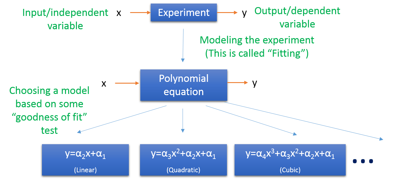
To keep things simple, we will consider only polynomial models.

Observed data and Least Squares estimation:

Suppose, an experiment is performed and the following data points are observed in the following table. The variable is the input to the experiment and is the output obtained. The input variable is often called “regressor”, “independent variable”, “manipulated variable”, etc. Similarly, the regression analysis jargon, the output variable or the observed variable is called “observed variable”, “explanatory variable”, “regressand” , “response variable” etc.

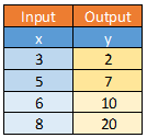
The aim of the experiment is to fit the experiment into a model with appropriate parameters. Once we know the model, we no longer need to perform the experiment to determine the output for any given arbitrary input. All we need to do is to use the model and generate the desired output.

Generic outline of an estimation algorithm:

We have a very small number of data points and it is four in our case. To illustrate the concept, we will choose linear model for parameter estimation. Higher order models will certainly give better performance. Remember!!! More the polynomial order, more is the number of parameters to be estimated and therefore the computational complexity will be more. It is necessary to strike a balance between the required performance and the model order.

We assume that the data points follow a linear trend. So, the linear model is chosen for the estimation problem.

Now the estimation problem simplifies to finding the parameters and . We can write the relationship between the observed variable and the input variable as

Next step is to solve for the above mentioned simultaneous equation based on least square error criterion. According to the criterion, the estimated values for and should produce minimum total squared error. Note the underlined words.

Let’s define the term – “error” for the above mentioned system of simultaneous equations. Error (which is a function of the model parameters) for one data point is the difference between the observed data and the data from the estimated model.

The sum of all squared errors is given by

Next step is to solve for and that gives minimum total squared error.

How do we find that? Employ calculus to find that. Separately take the partial derivative of with respect to and and set them to zero.

Solving the above simultaneous equations leads to the following solution

Thus, the model becomes

Solving using Matrices:

A system of simultaneous equations can be solved by Matrix manipulation. In DSP implementation of estimation algorithm, it is often convenient to work in matrix domain (especially when the number of data points becomes larger). Linear algebra is extensively used in implementing estimation algorithms on DSP processors.

The above mentioned set of data points can be represented in matrix notation as

Defining,

The set of simultaneous equations shrinks to

Given the criterion that the solution to the above equation must satisfy the minimum total squared error $latex S(\alpha)$,

The above equation simply denotes that the estimated parameter is the value of for which the error function attains the minimum.

The simultaneous equation mentioned above is a very simple case taken for illustration. For a generic case,

Usually, the above mentioned simultaneous equation may not have a unique solution. Unique solution exists if and only if all the columns of the matrix are linearly independent. Furthermore, the condition that the columns of matrix are linearly independent only means that they are orthogonal to each other. Thus the matrix is an orthogonal matrix.

For an orthogonal matrix, transpose and inverse are equivalent. That is,

Under this orthogonality condition, system of simultaneous equations become,

The solution is obtained by finding,

The aforementioned solution involves the computation of inverse of the matrix . Directly computing matrix inverses is cumbersome and computationally inefficient, especially when it comes to implementation in DSP, let alone the finite word length effects of fixed point processors. If the matrix , however large, has a very low condition number (i.e, well-conditioned) and if it is positive definite , then we can use Cholesky Decomposition to solve the equations.

This leads us to the next topic : “Cholesky Decomposition”

Rate this article: (6 votes, average: 3.00 out of 5)

Related Posts

[1]	An Introduction to Estimation Theory
[2]	Bias of an Estimator
[3]	Minimum Variance Unbiased Estimators (MVUE)
[4]	Maximum Likelihood Estimation
[5]	Maximum Likelihood Decoding
[6]	Probability and Random Process
[7]	Likelihood Function and Maximum Likelihood Estimation (MLE)
[8]	Score, Fisher Information and Estimator Sensitivity
[9]	Introduction to Cramer Rao Lower Bound (CRLB)
[10]	Cramer Rao Lower Bound for Scalar Parameter Estimation
[11]	Applying Cramer Rao Lower Bound (CRLB) to find a Minimum Variance Unbiased Estimator (MVUE)
[12]	Efficient Estimators and CRLB
[13]	Cramer Rao Lower Bound for Phase Estimation
[14]	Normalized CRLB - an alternate form of CRLB and its relation to estimator sensitivity
[15]	Cramer Rao Lower Bound (CRLB) for Vector Parameter Estimation
[16]	The Mean Square Error – Why do we use it for estimation problems
[17]	How to estimate unknown parameters using Ordinary Least Squares (OLS)
[18]	Essential Preliminary Matrix Algebra for Signal Processing
[19]	Why Cholesky Decomposition ? A sample case:
[20]	Tests for Positive Definiteness of a Matrix
[21]	Solving a Triangular Matrix using Forward & Backward Substitution
[22]	Cholesky Factorization - Matlab and Python
[23]	LTI system models for random signals – AR, MA and ARMA models
[24]	Comparing AR and ARMA model - minimization of squared error
[25]	Yule Walker Estimation
[26]	AutoCorrelation (Correlogram) and persistence – Time series analysis
[27]	Linear Models - Least Squares Estimator (LSE)
[28]	Best Linear Unbiased Estimator (BLUE)

Books by the author

Wireless Communication Systems in Matlab Second Edition(PDF) (180 votes, average: 3.62 out of 5) $14.99 – Add to Cart Checkout Added to cart	Digital Modulations using Python (PDF ebook) (134 votes, average: 3.56 out of 5) $14.99 – Add to Cart Checkout Added to cart	Digital Modulations using Matlab (PDF ebook) (136 votes, average: 3.63 out of 5) $14.99 – Add to Cart Checkout Added to cart
Hand-picked Best books on Communication Engineering Best books on Signal Processing