Key focus: AR, MA & ARMA models express the nature of transfer function of LTI system. Understand the basic idea behind those models & know their frequency responses.
How do you describe a complex, random signal—like the sound of a human voice or the fluctuating power of a fading channel—using only a few numbers?
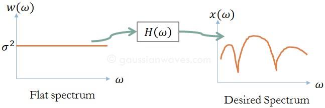
The secret lies in Signal Modeling. Instead of storing millions of samples, we model the signal as the output of a Linear Time-Invariant (LTI) system driven by white noise. By “shaping” the flat spectrum of white noise with a specific filter, we can recreate the statistical characteristics of almost any real-world random process.
Motivation
Let’s say we observe a real world signal x[n] that has a spectrum x[ɷ] (the spectrum can be arbitrary – bandpass, baseband etc..,). We would like to describe the long sequence of x[n] using very few parameters (application : Linear Predictive Coding (LPC) ). The modelling approach, described here, tries to answer the following two questions.
- Is it possible to model the first order (mean/variance) and second order (correlations, spectrum) statistics of the signal just by shaping a white noise spectrum using a transfer function ? (see Figure 1)
- Does this produce the same statistics (spectrum, correlations, mean and variance) for a white noise input ?
If the answer is “yes” to the above two questions, we can simply set the modeled parameters of the system and excite the system with white (flat) noise to produce the desired real world signal. This reduces the amount to data we wish to transmit in a communication system application.
LTI system model
In the model given below, the random signal x[n] is observed. Given the observed signal x[n], the goal here is to find a model that best describes the spectral properties of x[n] under the following assumptions
● x[n] is WSS (Wide Sense Stationary) and ergodic.
● The input signal to the LTI system is white noise following Gaussian distribution – zero mean and variance σ2.
● The LTI system is BIBO (Bounded Input Bounded Output) stable.

In the model shown above, the input to the LTI system is a white noise following Gaussian distribution – zero mean and variance σ2. The power spectral density (PSD) of the noise w[n] is
$$ S_{ww}(e^{j\omega}) = \sigma^2 $$
The noise process drives the LTI system with frequency response H(ejɷ) producing the signal of interest x[n]. The PSD of the output process is therefore,
$$ S_{xx}(e^{j\omega}) = \sigma^2 \left |H(e^{j\omega}) \right |^2 $$
The Generative Philosophy
In signal modeling, we assume a “black box” system. We feed it White Gaussian Noise ($w[n]$) with variance $\sigma^2$ and flat PSD, and it spits out our signal of interest ($x[n]$).
The Power Spectral Density (PSD) of the output is simply:
$$ S_{xx}(e^{j\omega}) = \sigma^2 \left| H(e^{j\omega}) \right|^2$$
Depending on the structure of the transfer function $H(e^{j\omega})$, we classify these models into three types: AR, MA, and ARMA.
Auto-Regressive (AR) Models: The “Peaky” Spectrum
An AR model is an all-pole system. It assumes the current output sample is a weighted sum of its own previous samples plus a new noise input.
Difference Equation:
$$x[n] = -\sum_{k=1}^{N} a_k x[n-k] + w[n]$$
Transfer Function:
$$H(z) = \frac{1}{1 + \sum_{k=1}^{N} a_k z^{-k}}$$
- Filter Type: IIR (Infinite Impulse Response).
- Key Strength: AR models are incredible at modeling resonant peaks (formants). If your signal has strong spectral peaks (like speech or motor vibrations), AR is your best friend.
- Stability Tip: For the signal to be stationary, all poles of $H(z)$ must lie inside the unit circle.

Moving Average (MA) Models: The “Null” Collector
An MA model is an all-zero system. The output is simply a weighted sum of current and past input noise samples.
Difference Equation:
$$x[n] = \sum_{k=0}^{M} b_k w[n-k]$$
Transfer Function:
$$H(z) = \sum_{k=0}^{M} b_k z^{-k}$$
- Filter Type: FIR (Finite Impulse Response).
- Key Strength: MA models excel at modeling spectral nulls (dips). If your channel has deep notches due to multi-path interference, an MA model captures that behavior perfectly.
- Stability: MA models are always BIBO stable because they have no poles (other than at the origin).

ARMA Models: The Best of Both Worlds
The Auto-Regressive Moving Average (ARMA) model is the most general form, combining both poles and zeros.
Transfer Function:
$$H(z) = \frac{\sum_{k=0}^{M} b_k z^{-k}}{1 + \sum_{k=1}^{N} a_k z^{-k}}$$
- When to use: Use ARMA for complex signals that have both sharp resonances (peaks) and deep cancellations (nulls). It provides the most compact description for sophisticated real-world spectra.

Why Does This Matter for Engineers?
Why go through the trouble of modeling?
- Compression (LPC): This is how cell phones work. Instead of sending the actual voice samples, the phone estimates the AR coefficients ($a_k$) of your vocal tract, sends those few numbers, and the receiver “synthesizes” the voice back using white noise.
- Spectral Estimation: If you have a noisy signal, fitting it to an AR model allows you to find its frequency components with much higher resolution than a standard FFT.
- System Identification: By looking at the output $x[n]$, we can “guess” the internal parameters of the system that created it.
Python Code Snippet: Visualizing AR vs. MA
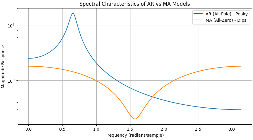
Following code demonstrates the difference between a “peaky” AR spectrum and a “notched” MA spectrum.
import numpy as np
import matplotlib.pyplot as plt
from scipy import signal

# AR Model (All-pole): Strong Resonances
a = [1, -1.5, 0.9] # Poles near the unit circle
w_ar, h_ar = signal.freqz([1], a)

# MA Model (All-zero): Deep Nulls
b = [1, 0, 0.8] # Zeros
w_ma, h_ma = signal.freqz(b, [1])

plt.figure(figsize=(10, 5))
plt.semilogy(w_ar, np.abs(h_ar), label='AR (All-Pole) - Peaky')
plt.semilogy(w_ma, np.abs(h_ma), label='MA (All-Zero) - Dips')
plt.title('Spectral Characteristics of AR vs MA Models')
plt.ylabel('Magnitude Response')
plt.xlabel('Frequency (radians/sample)')
plt.legend()
plt.grid()
plt.show()
AR vs. MA vs. ARMA: At a Glance
Following table consolidates the mathematical and practical differences between the three models in a format that’s easy to digest.
| Feature | Auto-Regressive (AR) | Moving Average (MA) | ARMA |
| System Type | All-Pole (IIR) | All-Zero (FIR) | Pole-Zero |
| Equation Logic | Output depends on past outputs. | Output depends on past inputs. | Combined feedback and feedforward. |
| Spectral Shape | Peaky. Best for modeling resonances. | Null-heavy. Best for modeling spectral dips. | Versatile. Can model both peaks and nulls. |
| Stability | Only stable if poles are inside the unit circle. | Always stable. | Only stable if poles are inside the unit circle. |
| Primary Use Case | Speech coding (LPC), Economics. | Multipath channel modeling. | Complex system identification. |
| Simplicity | High (Linear Yule-Walker equations). | Moderate (Non-linear estimation). | Low (High complexity). |
Summary of the Modeling Choice
Choosing between these models is often about parsimony—using the fewest parameters to describe the data.
- If your spectrum looks like a mountain range with sharp peaks, an AR model will describe it with just a few coefficients. Using an MA model for the same signal would require an impractically large number of terms.
- Conversely, if your spectrum has deep “valleys” or notches (common in wireless fading), the MA model is the most efficient choice.
- If the signal is a result of a physical process that both resonates and filters (like the human vocal tract combined with lip radiation), the ARMA model is the most accurate representation.
Next post: Comparing AR and ARMA model – minimization of squared error