Key focus: Discuss statistical measures for stochastic signals : mean, variance, skewness, kurtosis, histogram, scatterplot, cross-correlation and auto-correlation.
Deterministic and stochastic signals
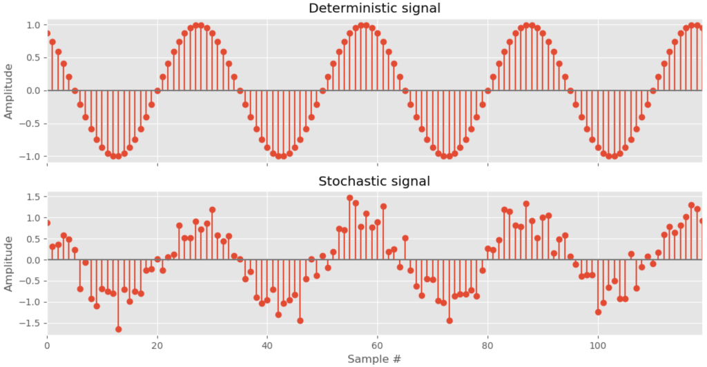
A deterministic signal is exactly predictable for the given time span of interest. It could be expressed using analytic form (example: x(t) = sin (2 π fc t) ).
Many of the signals that are encountered in real world signal processing applications cannot be expressed or predicted using analytic equations, because they have an element of uncertainty associated with them. As a consequence, such signals are characterized using statistical concepts. Therefore, these signals are outside the realm of deterministic signals and are classified as stochastic signals.
For example, we look at an electrical circuit and monitor the voltage across a resistor for a period of time. Under an applied electric field, atomic particles inside resister tend to randomly move and it manifests as heat. This random thermal motion causes random fluctuation in the voltage measured across the resistor. Therefore, the measured voltage can be characterized by a probability distribution and can be analyzed using statistical methods, but it cannot be predicted with precision. This is an example of signal that is stochastic function of time. Such functions usually evolve according to certain probabilistic laws and are assumed to be generated by an underlying stochastic process (thermal motion in the example above).
Given the amplitude of the stochastic voltage signal at time $latex t$, now we know, we cannot predict the value at t’. However, if we observed the signal for a sufficient amount of time, we can empirically determine its probability distribution based on which we should be able to answer questions like
- Given the amplitude of the voltage at time t, what is the average (expected or mean) of the voltage at time t’?
- How much can we expect the voltage at time t’, to fluctuate from the mean ? In other words, we are interested in the variance of the voltage at time t’.
- What is the probability that the voltage at t’ exceeds or falls below a certain threshold value ?
- How the voltages at times t and t’ are related ? In other words, we are interested in correlation.
Summary of descriptive statistical measures
Different statistical measures are available to gather, review, analyze and draw conclusions from stochastic signals. Some of the statistical measures are summarized below:
Quantitative measures of shape:
In many statistical analysis, the fundamental task is to get a general idea about the shape of a distribution and it is done by using moments.
Measure of central tendency – mean – the first moment:
Measures of central tendency attempt to identify the central position in the distribution of samples that make up the stochastic signal. Mean, mode and median are different measures of central tendency. In signal processing, we are mostly interested in computing mean which is the average of values of the given samples. Given a discrete random variable X with probability mass function pX(x) the mean is denoted by
\[\mu = E \left[ X\right] = \sum_{x: p_X(x) > 0} x p_X(x) \]Measure of dispersion – variance – the second moment:
Measures of dispersion describe how the values in the signal samples are spread out around a central location. Variance and standard deviation are some of the measures of dispersion. If the values are widely dispersed, the central location is said to be less representative of the values as a whole. If the values are tightly dispersed, the central location is considered more reliable.
For a discrete random variable X with probability mass function pX(x) , the variance (σX2) is given by the second central moment. The term central moment implies that this is measured relative to mean. For an electrical signal, the second moment is proportional to the average power.
\[\sigma_X^2 = E \left[ \left(X – \mu \right)^2\right] = \sum_{x: p_X(x) > 0} \left(x – \mu \right)^2 p_X(x) \]The square root of variance is standard deviation
\[\sigma_X = \sqrt{E \left[ \left(X – \mu \right)^2\right]}\]Figure 2, demonstrates the use of histogram for getting a visual perception of shape of the distribution of samples from two different stochastic signals. Though the signals look similar in nature in time domain, their histogram reveals different picture altogether. The central location (mean) of the first signal is around zero (no DC shift in the time domain view) and for the second signal the mean is at 0.75. The average power of first signal varies widely (histogram is widely spread out) compared to that of the second signal.

Higher order moments – skewness and kurtosis:
Further characterization of the shape of a distribution includes higher order moments : skewness and kurtosis. They identify anomalies and outliers in many signal processing applications.
Skewness provides a measure to quantify the presence of asymmetry in the shape of the distribution. Actually, skewness measures the relative size of the tails in a distribution. Presence of asymmetry manifests as non-zero value for the standardized third central moment. The term “standardized” stands for the normalization of the third central moment by σ3.
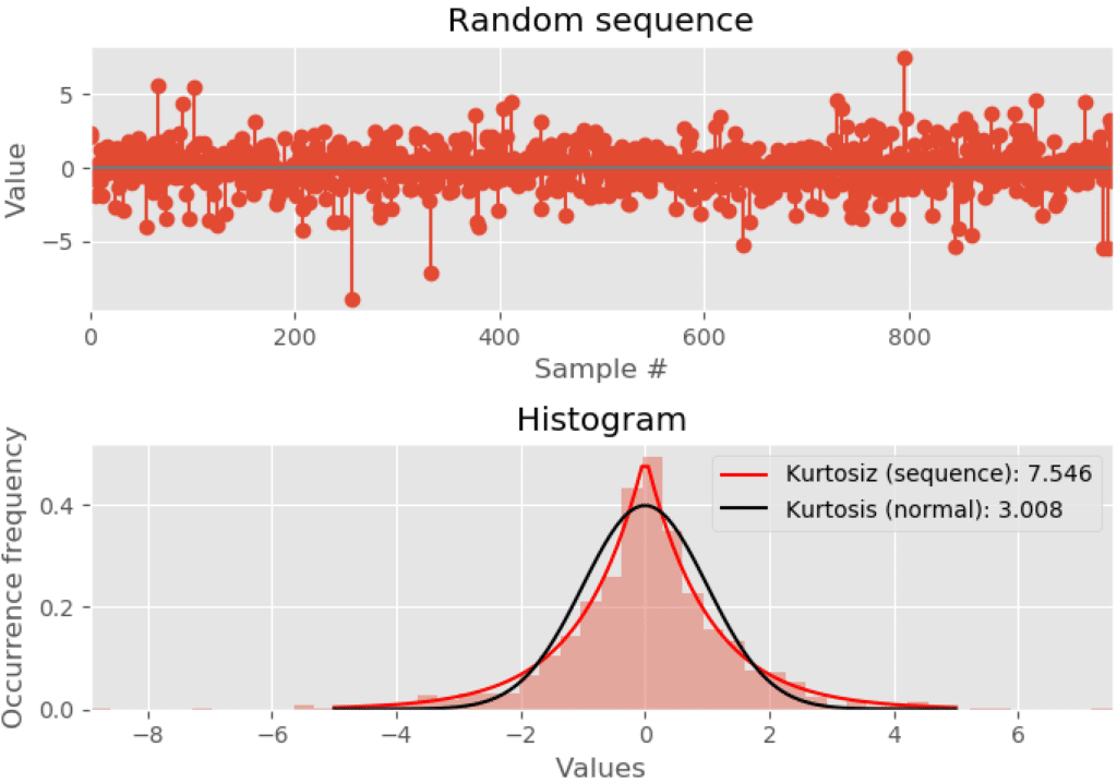
\[Skewness = \frac{E \left[ \left( X – \mu \right)^3 \right]}{\sigma^3}\]Kurtosis measures the amount of probability in the two tails of a distribution, relative to a normal distribution of same variance. Kurtosis is 3 for normal distribution (perfect bell shaped curve). If the kurtosis of a distribution is greater than 3, it implies that the tails are heavier compared to that of normal distribution. A value less than 3 for kurtosis implies lighter tails compared to that of the normal distribution. Essentially, kurtosis is a measure of outliers. Kurtosis is calculated as the standardized fourth central moment.
\[Kurtosis = \frac{E \left[ \left( X – \mu \right)^4 \right]}{\sigma^4}\]Measures of association
Statistics, such as measures of central tendency, dispersion and higher order moments, describe about a single distribution are called univariate statistics. If we are interested in the relationship between two or more variables, we have to move to at least the realm of bivariate statistics.
Measures of association, summarize the size of association between two variables. Most measures of associates are scaled to a range of values. For example, a measure of association can be construed to have a range 0 to 1, where the value 0 implies no relationship and a value of 1 implies perfect relationship between the two variables under study. In another case, the measure can range from -1 to 1, which can help us determine if the two variables have negative or positive relationship between each other.
Scatter plot
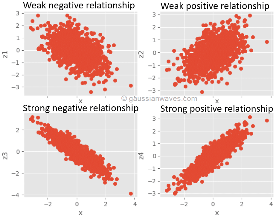
Scatter plot is a great way to visually assess the nature of relationship between two variables. Following figure contains the scatter plots between different stochastic signals, exhibiting different strengths of relationships between the signals.
Correlation
Correlation functions are commonly used in signal processing, for measuring the similarity of two signals. They are especially used in signal detection and pattern recognition.
Cross-correlation
Cross-correlation is commonly used for measuring the similarity between two different signals. In signal processing, cross-correlation measures the similarity of two waveforms as a function of time lags applied to one of the waveform.
For discrete-time waveforms – x[n] and y[n], cross correlation is defined as
\[Corr_{xy}[l] = \sum_{m=-\infty}^{\infty} x[n]^{\ast} y[n+l] = \sum_{m=-\infty}^{\infty} x[n-l]^{\ast} y[n]\]where, * denotes complex conjugate operation and l is the discrete time lags applied to one of the waveforms. That is, the cross-correlation can be calculated as the dot product of a sequence with each shifted version of another sequence.
Auto-correlation
Auto-correlation is the cross-correlation of a waveform/sequence with itself.
For discrete-time waveform – x[n], auto-correlation is defined as
\[Corr_{xx}[l] = \sum_{m=-\infty}^{\infty} x[n]^{\ast} x[n+l] = \sum_{m=-\infty}^{\infty} x[n-l]^{\ast} x[n] \]where, * denotes complex conjugate operation and l is the discrete time lags applied to the copy of the same waveform.
Correlation properties are useful for identifying/distinguishing a known bit sequence from a set of other possible known sequences. For example, in GPS technology, each satellite is assigned a unique 10-bit Gold code sequence (210 = 1023 possible combinations). Cross-correlation between different Gold code sequence is very low, since the Gold codes are orthogonal to each other. However, the auto-correlation of a Gold code is maximum at zero lag. The satellites are identified using these correlation properties of Gold codes. (I have described the hardware implementation of Gold codes, it can be accessed here).
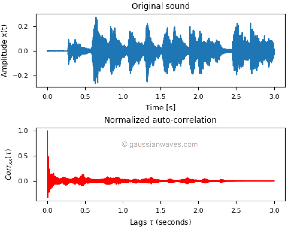
Following plots illustrate the application of auto-correlation for audio analysis. The auto-correlation of an audio signal will have a peak at zero lag (i.e, where there is no time shifting when computing the correlation) as shown in Figure 6. Figure 7 contains the same audio file that is synthetically processed to produce reverberation characteristics. By looking at the time series plot in Figure 7, we cannot infer anything. However, the auto-correlation plot reveals the reverberation characteristics embedded in the audio.

Rate this article: [ratings]
Books by the author
[table “23” not found /]

In time domain, the correlation coefficient can give information on the type and strength of correlation of the two signals. Do we have any such representation in frequency domain to define strength of correlation of two spectrums in a single value? other than obtaining bin by bin correlation by calculating their coherence?
Pearson Correlation coefficient for different domains are developed in the link below. The generalized case – full band squared Pearson correlation coefficient (SPCC) gives a single value and is defined for all frequencies.
https://link.springer.com/content/pdf/10.1007%2F978-3-642-00296-0.pdf
I couldn’t reply to the comment, so I’m posting a new comment.
Thank you, that was a good reference. I have one more question, since I’m new to this, I’m not sure if the following question makes any sense at all, nonetheless would like to clarify. In case if we have only absolute value of two frequency spectrums, in that case, would it be right to simply calculate the Pearson correlation coefficient considering the two spectrums as sets of random variables, if their bin resolution is identical.
Absolute values alone do not contain all the information in the frequency domain.
Yes, that is right. However, the absolute values will give an indication of the magnitude of the different frequency components present in the signal, so would it be right to correlate the two spectrums as datasets, just to draw conclusion on how closely magnitude of each bin is correlated?