Line code – demonstration in Matlab and Python

Line code is the signaling scheme used to represent data on a communication line. There are several possible mapping schemes available for this purpose. Lets understand and demonstrate line code and PSD (power spectral density) in Matlab & Python.

Line codes – requirements

When transmitting binary data over long distances encoding the binary data using line codes should satisfying following requirements.

• All possible binary sequences can be transmitted.
• The line code encoded signal must occupy small transmission bandwidth, so that more information can be transmitted per unit bandwidth.
• Error probability of the encoded signal should be as small as possible
• Since long distance communication channels cannot transport low frequency content (example : DC component of the signal , such line codes should eliminate DC when encoding). The power spectral density of the encoded signal should also be suitable for the medium of transport.
• The receiver should be able to extract timing information from the transmitted signal.
• Guarantee transition of bits for timing recovery with long runs of 1s and 0s in the binary data.
• Support error detection and correction capability to the communication system.

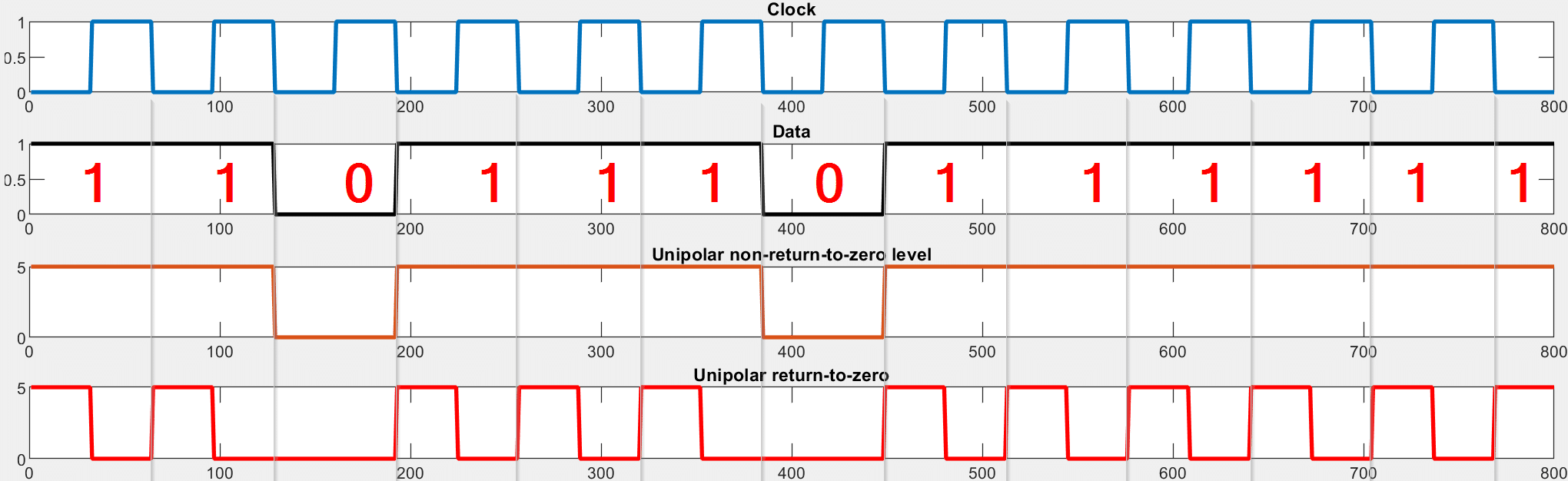
Unipolar Non-Return-to-Zero (NRZ) level and Return-to-Zero (RZ) level codes

Unipolar NRZ(L) is the simplest of all the line codes, where a positive voltage represent binary bit 1 and zero volts represents bit 0. It is also called on-off keying.

In unipolar return-to-zero (RZ) level line code, the signal value returns to zero between each pulse.

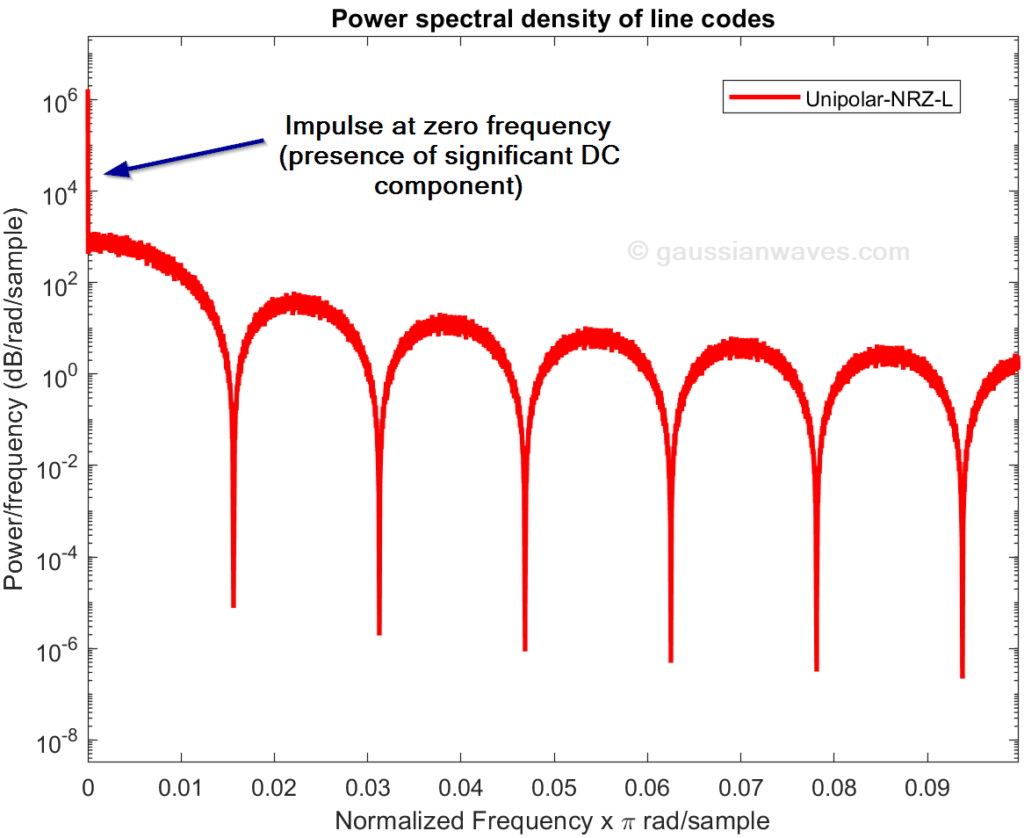
For both unipolar NRZ and RZ line coded signal, the average value of the signal is not zero and hence they have a significant DC component (note the impulse at zero frequency in the power spectral density (PSD) plot).

The DC impulses in the PSD do not carry any information and it also causes the transmission wires to heat up. This is a wastage of communication resource.

Unipolar coded signals do not include timing information, therefore long runs of 0s and 1s can cause loss of synchronization at the receiver.

Bipolar Non-Return-to-Zero (NRZ) level code

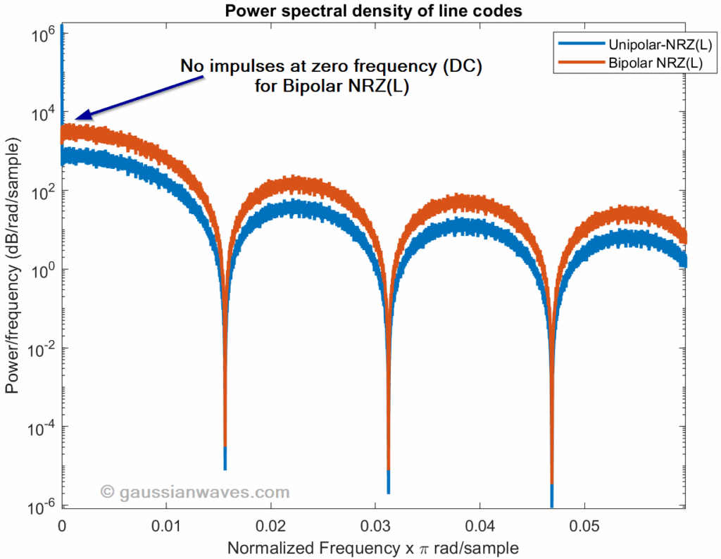
In bipolar NRZ(L) coding, binary bit 1 is mapped to positive voltage and bit 0 is mapped to negative voltage. Since there are two opposite voltages (positive and negative) it is a bipolar signaling scheme.

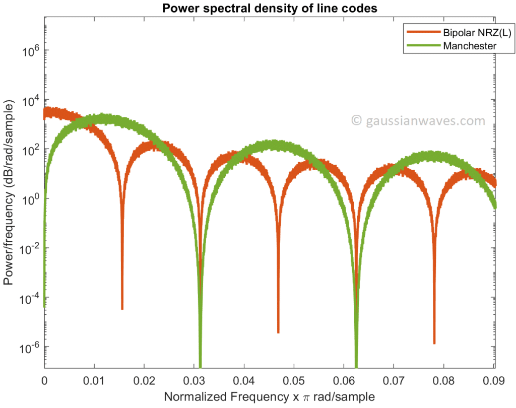
Evident from the power spectral densities, the bipolar NRZ signal is devoid of a significant impulse at the zero frequency (DC component is very close to zero). Furthermore, it has more power than the unipolar line code (note: PSD curve for bipolar NRZ is slightly higher compared to that of unipolar NRZ). Therefore, bipolar NRZ signals provide better signal-to-noise ratio (SNR) at the receiver.

Bipolar NRZ signal lacks embedded clock information, which posses synchronization problems at the receiver when the binary information has long runs of 0s and 1s.

Alternate Mark Inversion (AMI)

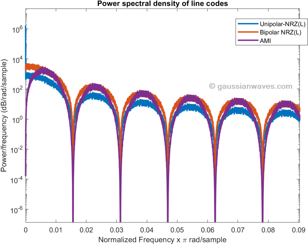
AMI is a bipolar signaling method, that encodes binary 0 as 0 Volt and binary 1 as +ve and -ve voltage (alternating between successive 1s).

AMI eliminates DC component. Evident from the PSD plots below, AMI has reduced bandwidth (narrower bumps) and faster roll-offs compared to unipolar and bipolar NRZ line codes.

It has inbuilt error detection mechanism: a bit error results in violation of bipolar signaling. It has guaranteed timing transitions even for long runs of 1s and 0s.

Manchester encoding

In Manchester encoding, the signal for each binary bit contains one transition. For example, bit 0 is represented by a transition from negative to positive voltage and bit 1 is represented by transitioning from one positive to negative voltage. Therefore, it is considered to be self clocking and it is devoid of DC component.

Digitally Manchester encoding can be implemented by XORing the binary data and the clock, followed by mapping the output to appropriate voltage levels.

From the PSD plot, we can conclude that Manchester encoded signal occupies twice the bandwidth of Bipolar NRZ(L) encoded signal.

Matlab script

In this script, lines codes are simulated and their power spectral density (PSD) are plotted using pwelch command.

%Simulate line codes and plot power spectral densities (PSD)
%Author: Mathuranathan Viswanathan
clearvars; clc;
L = 32; %number of digital samples per data bit
Fs = 8*L; %Sampling frequency
voltageLevel = 5; %peak voltage level in Volts
data = rand(10000,1)>0.5; %random 1s and 0s for data
clk = mod(0:2*numel(data)-1,2).'; %clock samples

ami = 1*data; previousOne = 0; %AMI encoding
for ii=1:numel(data)
    if (ami(ii)==1) && (previousOne==0)
        ami(ii)= voltageLevel;
        previousOne=1;
    end 
    if (ami(ii)==1) && (previousOne==1)
        ami(ii)= -voltageLevel;
        previousOne = 0;
    end    
end

%converting the bits to sequences and mapping to voltage levels
clk_sequence=reshape(repmat(clk,1,L).',1,length(clk)*L);
data_sequence=reshape(repmat(data,1,2*L).',1,length(data)*2*L);
unipolar_nrz_l = voltageLevel*data_sequence;
nrz_encoded = voltageLevel*(2*data_sequence - 1);
unipolar_rz = voltageLevel*and(data_sequence,not(clk_sequence));
ami_sequence = reshape(repmat(ami,1,2*L).',1,length(ami)*2*L);
manchester_encoded = voltageLevel*(2*xor(data_sequence,clk_sequence)-1);

figure; %Plot signals in time domain 
subplot(7,1,1); plot(clk_sequence(1:800)); title('Clock');
subplot(7,1,2); plot(data_sequence(1:800)); title('Data')
subplot(7,1,3); plot(unipolar_nrz_l(1:800)); title('Unipolar non-return-to-zero level')
subplot(7,1,4); plot(nrz_encoded(1:800)); title('Bipolar Non-return-to-zero level')
subplot(7,1,5); plot(unipolar_rz(1:800)); title('Unipolar return-to-zero')
subplot(7,1,6); plot(ami_sequence(1:800)); title('Alternate Mark Inversion (AMI)')
subplot(7,1,7); plot(manchester_encoded(1:800)); title('Manchester Encoded - IEEE 802.3')

figure; %Plot power spectral density
ns = max(size(unipolar_nrz_l));
na = 16;%averaging factor to plot averaged welch spectrum
w = hanning(floor(ns/na));%Hanning window
%Plot Welch power spectrum using Hanning window
[Pxx1,F1] = pwelch(unipolar_nrz_l,w,[],[],1,'onesided');
[Pxx2,F2] = pwelch(nrz_encoded,w,[],[],1,'onesided'); 
[Pxx3,F3] = pwelch(unipolar_rz,w,[],[],1,'onesided'); 
[Pxx4,F4] = pwelch(ami_sequence,w,[],[],1,'onesided'); %
[Pxx5,F5] = pwelch(manchester_encoded,w,[],[],1,'onesided'); 

semilogy(F1,Pxx1,'DisplayName','Unipolar-NRZ-L');hold on;
semilogy(F2,Pxx2,'DisplayName','Bipolar NRZ(L)');
semilogy(F3,Pxx3,'DisplayName','Unipolar-RZ');
semilogy(F4,Pxx4,'DisplayName','AMI'); 
semilogy(F5,Pxx5,'DisplayName','Manchester');
legend();

Python code

Check out the python code in my Google Colab

Rate this article: (19 votes, average: 3.89 out of 5)

Books by the author

Wireless Communication Systems in Matlab Second Edition(PDF) (180 votes, average: 3.62 out of 5) $14.99 – Add to Cart Checkout Added to cart	Digital Modulations using Python (PDF ebook) (134 votes, average: 3.56 out of 5) $14.99 – Add to Cart Checkout Added to cart	Digital Modulations using Matlab (PDF ebook) (136 votes, average: 3.63 out of 5) $14.99 – Add to Cart Checkout Added to cart
Hand-picked Best books on Communication Engineering Best books on Signal Processing