Code Division Multiple Access (CDMA) systems multiplex users over identical time and frequency slots. Separation occurs entirely in the code domain.
Fifty people talk at once in one room. Each pair speaks a different language, so you still follow your friend.
That is CDMA. All users share the same frequency and the same time, and each user gets a code that works like a private language. Four code families make it work.
1. What spreading actually does: cdma
Say you want to send the bit +1. Instead of sending it as one long pulse of duration $T_b$, you chop it into 8 shorter pulses, called chips, each lasting
$$T_c = \frac{T_b}{SF}\,$$
and multiply them by a code like − + + + + − − −.
If $b(t) in \lbrace +1, -1\rbrace $ is your data and $c(t) in \lbrace +1, -1\rbrace $ is the code, the transmitted signal is just their product:
$$s(t) = b(t)\,c(t).$$
On the other end, the receiver multiplies by the same code. Since $c^2(t) = 1$ for every chip, the code cancels:
$$s(t)\,c(t) = b(t)\,c^2(t) = b(t).$$
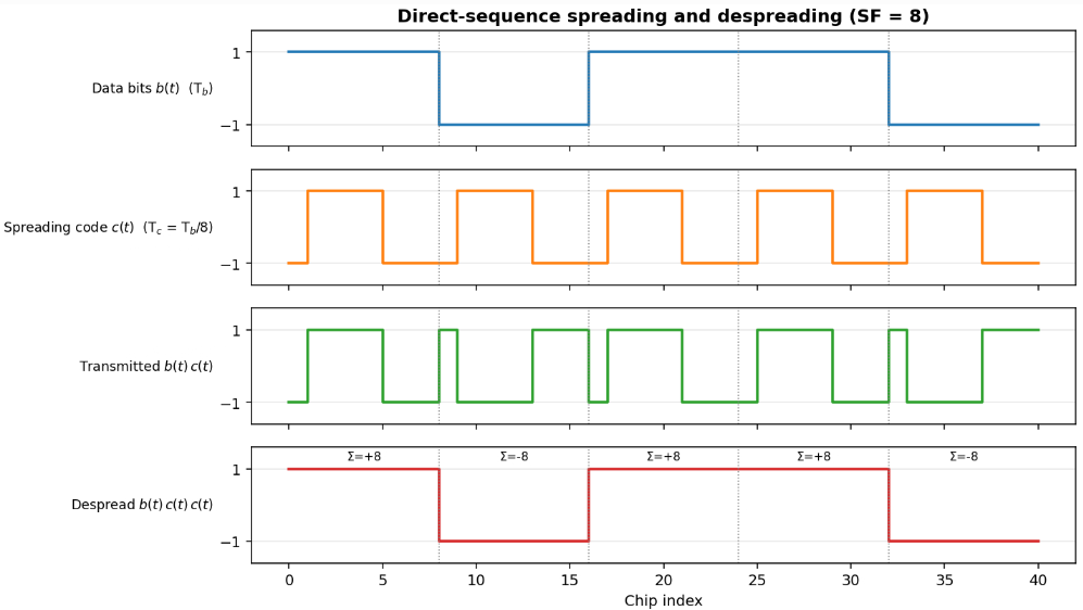
The number of chips per bit is called the spreading factor, or $SF$. Here $SF = 8$.
So why does this separate users? Imagine someone else’s signal also lands on your receiver. In discrete chips, for one bit period, the receiver gets
$$r[n] = b_1\,c_1[n] + b_2\,c_2[n], \qquad n = 0, \dots, SF-1,$$
where user 1 is you and user 2 is someone else. Multiply by your code and add up the chips:
$$z = \sum_{n=0}^{SF-1} r[n]\,c_1[n] = \overbrace{b_1 \cdot SF}^{\text{your bit}} + \overbrace{b_2 \sum_{n=0}^{SF-1} c_2[n]\,c_1[n]}^{\text{interference}}.$$
Your bit comes through with a weight of $SF$. The other user only gets through as much as the two codes look alike. That gap between “my signal” and “everyone else” is the processing gain:
$$G_p = 10 \log{10}(SF) \text{dB}. $$
With $SF = 8$ you get about 9 dB. With $SF = 128$, about 21 dB.
Keep one question in your head for the rest of this post: how much do two codes look like each other? That’s exactly the sum in the interference term. We call it the correlation, and since codes can arrive with a time offset $\tau$, we look at it for every shift:
$$R_{xy}(\tau) = \sum_{n=0}^{N-1} x[n]\, y[(n+\tau) \bmod N].$$
When $x = y$ this is the autocorrelation, and when $x \neq y$ it’s the cross-correlation. A big number means the codes look alike, which is bad. Zero means they’re completely different, or orthogonal, which is exactly what we want.
2. Walsh codes
Walsh codes are built with a simple rule: copy, and copy with a flip. Start with a $1 times 1$ matrix and keep doubling:
$$H_1 = \begin{bmatrix} +1 \end{bmatrix}\, \qquad H_{2N} = \begin{bmatrix} H_N & H_N \cr H_N & -H_N \end{bmatrix}.$$
Written out, the first few steps look like this:
+   →   + +    →   + + + +
            + −          + − + −
                            + + − −
                            + − − +
Each row is a code. Keep going and you get 8, 16, 64 codes, as many as you need.
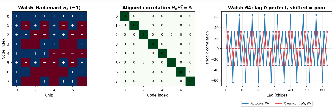
The middle panel is the reason people love these codes. Each code matches itself, and every pair of different codes gives exactly zero. In matrix form:
$$H_N\,H_N^{T} = N\,I_N \quad\Longleftrightarrow\quad \sum_{n=0}^{N-1} w_i[n]\,w_j[n] = \begin{cases} N, & i = j \cr 0\, & i \neq j \end{cases}$$
Not “small”, zero. Try two rows from above with a pencil:
Row 2:    +  −  +  −
Row 3:    +  +  −  −
Product:  +  −  −  +    → sum = 0
So 64 users on 64 Walsh codes don’t bother each other at all.
Now look at the right panel. The zero only holds at $\tau = 0$. Shift one code by a single chip and
$$R_{w_5 w_6}(\tau) \neq 0 \quad \text{for } \tau \neq 0,$$
and for this pair it goes as high as 32, half of a full match of 64.
Walsh codes are like a marching band. When everyone is on the beat, the formation is perfect. When one person is half a step late, the whole thing looks wrong.
That tells you where Walsh codes belong. On the downlink, one tower sends everyone’s signal from one clock, so they all leave in perfect step. On the uplink, every phone sits at a different distance with its own clock, so nothing lines up. That’s why 2G CDMA (IS-95) uses 64 Walsh codes on the downlink. Code 0 is the pilot, a beacon every phone listens to, and the others carry sync, paging and calls.
3. PN sequences
Here’s a problem I skipped over. Before a phone can use any Walsh code, it has to know exactly when each chip starts. It also has to figure out which tower it’s listening to. Walsh codes are no help here. Shifted copies of them look too much alike.
What we want is a code that matches itself at one position and looks like noise everywhere else.
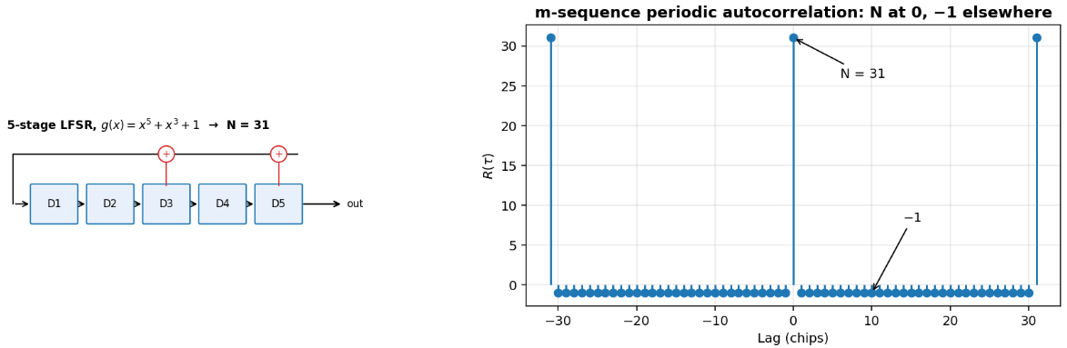
The usual way to make one is a linear feedback shift register, or LFSR. It’s just a row of memory boxes. On every clock tick, the bits shift one place to the right, the bit that drops off the end is your output, and a couple of chosen boxes are XORed together and fed back in at the start.
For the register in Figure 3, with feedback from boxes 3 and 5, each new bit is
$$a_n = a_{n-3} \oplus a_{n-5},$$
where $\oplus$ is XOR (addition mod 2). We describe the taps with a polynomial whose powers list the tapped boxes:
$$g(x) = 1 + x^3 + x^5.$$
If $g(x)$ is a primitive polynomial, an $n$-box register cycles through every possible non-zero state before it repeats. That gives you the longest pattern you can get from it,
$$N = 2^n – 1 \, \text{chips}\,$$
which is why it’s called a maximal-length sequence, or m-sequence. Five boxes give you $2^5 – 1 = 31$ chips. Forty-two boxes give you $2^{42} – 1 \approx 4.4 \times 10^{12}$.
The right side of Figure 3 is the part I want you to stare at. Map the bits to $\pm 1$ with $x[n] = 1 – 2a_n$, and the autocorrelation takes only two values:
$$R_{xx}(\tau) = \begin{cases} N, & \tau \equiv 0 \pmod N \cr -1\, & \text{otherwise} \end{cases}$$
At zero shift you get 31. At every other shift you get −1, which is basically nothing. It behaves like a key that only turns in one position. The phone slides its own copy of the code along until that spike pops up, and now it knows the timing exactly.
The pattern also looks random. Out of $2^n – 1$ chips, there are $2^{n-1}$ ones and $2^{n-1} – 1$ zeros, so it’s almost perfectly balanced. Its runs of ones and zeros look like coin flips. But it’s completely predictable, because the same register always gives the same output. Hence the name pseudo-noise, or PN.
IS-95 does something clever with this. Every tower uses the same short PN code of length $2^{15}$, but each one starts it at a different time offset. There are 512 offsets, each 64 chips apart, and the offset is the tower’s ID. There’s also a second, much longer PN code that gives each user some privacy. Its period is
$$\frac{2^{42} – 1}{1.2288 \times 10^{6} \text{chips/s}} \approx 3.58 \times 10^{6} \text{s} \approx 41 \text{ days}.$$
4. Gold codes
So far we have Walsh codes, which need perfect timing, and PN sequences, which are great for finding timing. But what about the uplink, where users are out of step and we need lots of codes that don’t clash?
You might think: give everyone a different m-sequence. The trouble is that two different m-sequences can correlate quite badly with each other.
In 1967, Robert Gold found a way around this. Take two specific m-sequences $a$ and $b$ that form a preferred pair. XOR them together. Then shift $b$ by a chip and XOR again. Keep doing that for every possible shift. If $T^k b$ means “$b$ shifted by $k$ chips”, the full family is
$$\mathcal{G}(a, b) = \left\lbrace \, a,\; b,\; a \oplus b,\; a \oplus T b,\; a \oplus T^2 b,\; \dots,\; a \oplus T^{N-1} b \,\right\rbrace .$$
That’s $N$ combinations plus the two originals, so
$$|\mathcal{G}| = N + 2 = 2^n + 1 \text{codes}.$$
With length 31 you get 33 codes.
A small detail that makes the maths easier: once you map bits to $\pm 1$, XOR turns into ordinary multiplication,
$$1 – 2\,(a_n \oplus b_n) = (1 – 2a_n)(1 – 2b_n).$$
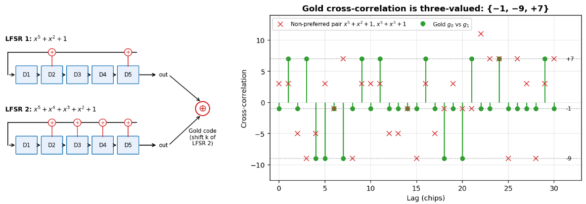
The green dots are the whole point. However you shift them, two Gold codes only ever correlate to one of three values:
$$R_{xy}(\tau) \in \lbrace \, -1,\; -t(n),\; t(n) – 2 \,\rbrace \, \qquad t(n) = \begin{cases} 1 + 2^{(n+1)/2}\, & n \text{ odd} \cr 1 + 2^{(n+2)/2}\, & n \text{ even} \end{cases}$$
For $n = 5$, $t(5) = 1 + 2^3 = 9$, so the values are $\lbrace -1, -9, +7\rbrace $, which is exactly what the green dots show. Compared with a full match of 31, the worst case is
$$\frac{|R_{xy}|_{max}}{N} = \frac{9}{31} \approx 0.29.$$
That’s small, and more importantly it’s guaranteed. The red crosses show a pair that isn’t preferred. The values wander all over the place and hit +11.
That guarantee is why Gold codes turn up everywhere. Every GPS satellite has its own Gold code of length $2^{10} – 1 = 1023$, which is how your phone tells them apart. In 3G, each cell gets one, and so does each phone on the uplink. Even 5G, which doesn’t use CDMA at all, still uses a Gold-sequence generator to make its scrambling bits and reference signals. It’s built from two length-31 registers (3GPP TS 38.211, Section 5.2.1):
$$c(n) = \big(x_1(n + N_c) + x_2(n + N_c)\big) \bmod 2, \qquad N_c = 1600\,$$
$$x_1(n+31) = \big(x_1(n+3) + x_1(n)\big) \bmod 2\,$$
$$x_2(n+31) = \big(x_2(n+3) + x_2(n+2) + x_2(n+1) + x_2(n)\big) \bmod 2.$$
5. OVSF codes
By the time 3G came along, a new problem showed up. In 2G almost everyone was on a voice call at roughly the same rate. In 3G, one person might be streaming video while the person next to them sends a text. With a fixed chip rate $R_c$, the data rate depends on the spreading factor:
$$R_b = \frac{R_c}{SF}.$$
So the video user needs a smaller $SF$. Can you mix short and long codes and still keep them orthogonal?
You can, with OVSF codes (orthogonal variable spreading factor). They grow like a family tree, where every code has two children:
$$C_{2SF\,,2k} = \begin{bmatrix} C_{SF,k} & C_{SF,k} \end{bmatrix}\, \qquad C_{2SF\,,2k+1} = \begin{bmatrix} C_{SF,k} & -C_{SF,k} \end{bmatrix}.$$
In words: one child is the parent written twice, and the other is the parent followed by a flipped copy of itself.
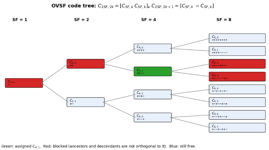
There’s really only one rule to remember: a code is orthogonal to everything in the tree except its own ancestors and descendants.
So once someone is using $C_{4,1}$, nobody else can have its parent $C_{2,0}$ or its children $C_{8,2}$ and $C_{8,3}$. Everything on the other branches is fine.
I like to think of it as slicing a pizza. If you take a quarter, you’ve also taken the two eighths inside that quarter. A code with spreading factor $SF$ uses up $1/SF$ of the tree, and the total can never go over the whole pizza:
$$\sum_{\text{assigned codes}} \frac{1}{SF_i} le 1.$$
A video user at $SF = 4$ takes $1/4$ of everything. A voice user at $SF = 128$ takes $1/128$, barely anything.
6. How it all fits together
Here’s the part that ties everything up. Real systems don’t pick one code family. They use two layers at once, a bit like a postal address.
The channelization code (Walsh or OVSF) is the apartment number. It keeps users in the same cell apart and sets each one’s data rate. The scrambling code (PN or Gold) is the street address. It keeps neighbouring cells apart, and users who aren’t in step, without using any extra bandwidth.
Mathematically, both are just multiplied on, chip by chip. For user $k$ in a cell:
$$s_k[n] = b_k[n]\; \overbrace{C_{SF,k}[n]}^{\text{channelization}}\; \overbrace{S_{\text{cell}}[n]}^{\text{scrambling}}.$$
The scrambling code runs at the chip rate, so it doesn’t change the bandwidth. Only the spreading factor does.
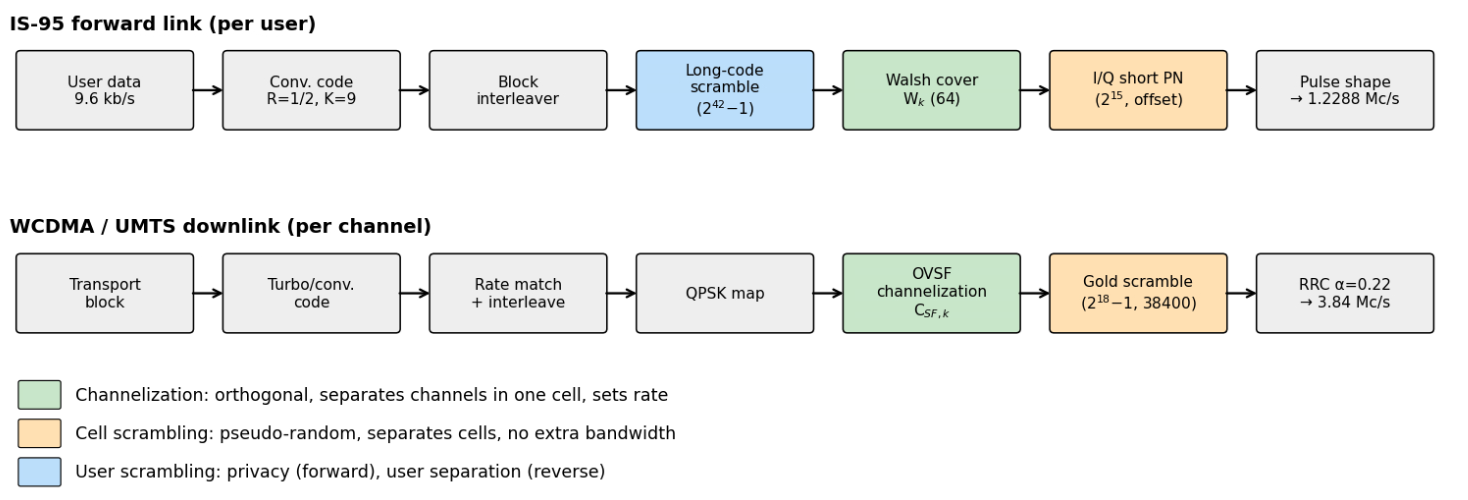

If you trace either chain from left to right, the data gets error-correction coding and interleaving first. Then the green block gives it its apartment number, and the orange block stamps the cell’s street address on top before it goes out.
Try it yourself
I’d really encourage you to run this. It’s a few lines of Python, and it checks the two big claims from this post: $H_8 H_8^T = 8 I$ for Walsh codes, and the three correlation values for Gold codes.
import numpy as np
def walsh(n):
    """Return n Walsh codes of length n (n = 1, 2, 4, 8, ...)."""
    H = np.array([[1]])
    while len(H) < n:
        H = np.block([[H, H], [H, -H]])
    return H
def lfsr(taps, n):
    """Return an m-sequence (0/1) from an n-box shift register."""
    state, out = [1] * n, []
    for _ in range(2**n - 1):
        out.append(state[-1])
        fb = 0
        for t in taps:
            fb ^= state[t - 1]
        state = [fb] + state[:-1]
    return np.array(out)
# Walsh: 8 on the diagonal, 0 everywhere else
H = walsh(8)
print(H @ H.T)
# Gold: only three correlation values
a, b = lfsr([2, 5], 5), lfsr([2, 3, 4, 5], 5)
g0 = 1 - 2 * a
g1 = 1 - 2 * (a ^ np.roll(b, 1))
print({int(np.dot(g0, np.roll(g1, k))) for k in range(31)}) # {-9, -1, 7}Once it runs, try changing [2, 3, 4, 5] to [3, 5]. That breaks the preferred pair, and you’ll see new correlation values show up. It’s a nice way to convince yourself the “preferred” part actually matters.
Quick recap
| Code | Good at | Not so good at | Where you’ll see it |
|---|---|---|---|
| Walsh | Zero interference at $\tau = 0$ | Needs perfect timing | Downlink channels |
| PN (m-sequence) | Finding timing, $R(\tau) = -1$ off-peak | Different PN codes can clash | Tower ID, user privacy |
| Gold | $2^n + 1$ codes, bounded clash | Not exactly zero | GPS, 3G, 5G sequences |
| OVSF | Mixing data rates, $R_b = R_c / SF$ | Blocks whole branches | 3G data |
A few questions to check yourself
- A system uses $SF = 64$. What’s the processing gain?
- Why can’t the uplink rely on Walsh codes alone?
- In the OVSF tree, $C_{8,5}$ is in use. Which $SF = 4$ code is now blocked?
- A Gold code family uses $n = 7$. How many codes are there, and what are the three correlation values?
Answers - $G_p = 10\log_{10}(64) \approx 18$ dB.
- Uplink signals arrive out of step, and $R_{w_i w_j}(\tau) \neq 0$ for $\tau \neq 0$.
- $C_{4,2}$, since $C_{8,5} = [,C_{4,2}\;; -C_{4,2}\,]$.
- $2^7 + 1 = 129$ codes. With $t(7) = 1 + 2^4 = 17$, the values are $\lbrace -1, -17, +15\rbrace $.
If you want to keep going, have a look at Walsh–Hadamard codes in Matlab, the spread spectrum intro, or play with the Eb/N0 ↔ SNR converter to see where processing gain fits in a link budget.
Keep learning
- Walsh–Hadamard codes — generate the matrix and simulate in Matlab
- Spread Spectrum Communications – Intro
- 3GPP TDL channel calculator: see how multipath delay spread breaks Walsh orthogonality
- Eb/N0, Es/N0 and SNR converter: processing gain in a link budget
Go further with the ebooks: the Digital Modulations ebooks include full Matlab/Python projects on spreading, despreading, and BER. Compare all books.
References
IS-GPS-200, Navstar GPS Space Segment / Navigation User Segment Interfaces.
TIA/EIA IS-95-A, Mobile Station–Base Station Compatibility Standard for Dual-Mode Wideband Spread Spectrum Cellular System, 1995.
3GPP TS 25.213, Spreading and modulation (FDD).
3GPP TS 38.211, NR; Physical channels and modulation, §5.2.1 Pseudo-random sequence generation.
R. Gold, “Optimal binary sequences for spread spectrum multiplexing,” IEEE Trans. Inf. Theory, vol. 13, no. 4, pp. 619–621, Oct. 1967.