Binomial random variable, a discrete random variable, models the number of successes in $latex n$ mutually independent Bernoulli trials, each with success probability $latex p$. The term Bernoulli trial implies that each trial is a random experiment with exactly two possible outcomes: success and failure. It can be used to model the total number of bit errors in the received data sequence of length $latex n$ that was transmitted over a binary symmetric channel of bit-error probability $latex p$.
Generating binomial random sequence in Matlab
Let X denotes the total number of successes in $latex n$ mutually independent Bernoulli trials. For ease of understanding, let’s denote success as ‘1’ and failure as ‘0’. Suppose if a particular outcome of the experiment contains $latex x$ ones and $latex n-x$ zeros (example outcome: 1011101), the probability mass function↗ of $latex X$ is given by
$latex f_X(x) = \binom{n}{x} p^x \left( 1-p \right)^{n-x} \quad , x \in {0,1,2, \cdots,n}&s=2$
A binomial random variable can be simulated by generating $latex n$ independent Bernoulli trials and summing up the results.
function X = binomialRV(n,p,L)
%Generate Binomial random number sequence
%n - the number of independent Bernoulli trials
%p - probability of success yielded by each trial
%L - length of sequence to generate
X = zeros(1,L);
for i=1:L,
   X(i) = sum(bernoulliRV(n,p));
end
end
Following program demonstrates how to generate a sequence of binomially distributed random numbers, plot the estimated and theoretical probability mass functions for the chosen parameters (Figure 1).
n=30; p=1/6; %number of trails and success probability
X = binomialRV(n,p,10000);%generate 10000 bino rand numbers
X_pdf = pdf('Binomial',0:n,n,p); %theoretical probility density
histogram(X,'Normalization','pdf'); %plot histogram
hold on; plot(0:n,X_pdf,'r'); %plot computed theoreical PDF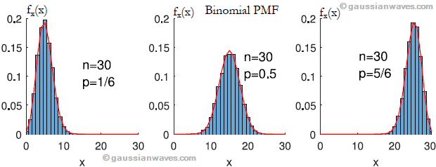
PMF sums to unity
Let’s verify theoretically, the fact that the PMF of the binomial distribution sums to unity. Using the result of Binomial theorem↗,
$latex 1 = 1^n = \left( p+1 -p \right)^n = \displaystyle{ \sum_{x=0}^{n}\binom{n}{x} p^x \left( 1-p \right)^{n-x}} &s=2$
Mean and variance
The mean number of success in a binomial distribution is
$latex \mu = E[X] = np &s=2$
The variance is
$latex \sigma^2 = E\left[ \left(X – \mu \right)^2 \right] = np (1-p) &s=2$
Rate this article: [ratings]
Topics in this chapter
[table “33” not found /]Books by the author
[table “23” not found /]