Key focus: Know how to generate a Chirp signal, compute its Fourier Transform using FFT and power spectral density (PSD) in Matlab & Python.
[table “47” not found /]Introduction
All the signals discussed so far do not change in frequency over time. Obtaining a signal with time-varying frequency is of main focus here. A signal that varies in frequency over time is called “chirp”. The frequency of the chirp signal can vary from low to high frequency (up-chirp) or from high to low frequency (low-chirp).
Observation
Chirp signals/signatures are encountered in many applications ranging from radar, sonar, spread spectrum, optical communication, image processing, doppler effect, motion of a pendulum, as gravitation waves, manifestation as Frequency Modulation (FM), echo location [1] etc.
Mathematical Description:
A linear chirp signal sweeps the frequency from low to high frequency (or vice-versa) linearly. One approach to generate a chirp signal is to concatenate a series of segments of sine waves each with increasing(or decreasing) frequency in order. This method introduces discontinuities in the chirp signal due to the mismatch in the phases of each such segments. Modifying the equation of a sinusoid to generate a chirp signal is a better approach.
The equation for generating a sinusoidal (cosine here) signal with amplitude A, angular frequency $latex \omega_0$ and initial phase $latex \phi$ is
$latex x(t)=A cos(\omega_0 t + \phi ) \quad\quad (1) &s=1$
This can be written as a function of instantaneous phase
$latex x(t)= A cos(\theta (t)) = A cos ( \omega_0 t+ \phi ) = A cos ( 2 \pi f_0 t+ \phi ) \quad (2) &s=1$
where $latex \theta (t) = \omega_0 t+ \phi$ is the instantaneous phase of the sinusoid and it is linear in time. The time derivative of instantaneous phase $latex \theta(t)$ is equal to the angular frequency $latex \omega$ of the sinusoid – which in case is a constant in the above equation.
$latex \omega_0 = \frac{d}{dt} \theta (t) \quad\quad (3)&s=1$
Instead of having the phase linear in time, let’s change the phase to quadratic form and thus non-linear.
$latex \theta(t) = 2 \pi \alpha t^2 + 2 \pi f_0 t + \phi \quad\quad (4) &s=1$
for some constant $latex \alpha$.
Therefore, the equation for chirp signal takes the following form,
$latex x(t) = A cos(\theta(t)) = A cos( 2 \pi \alpha t^2 + 2 \pi f_0 t + \phi ) \quad (5)&s=1$
The first derivative of the phase, which is the instantaneous angular frequency becomes a function of time, which is given by
$latex \omega_i(t)=\frac{d}{dt} \theta (t) = 4 \pi \alpha t + 2 \pi f_0 \quad\quad (6)&s=1$
The time-varying frequency in Hertz is given by
$latex f_i (t) = 2 \alpha t + f_0 \quad\quad (7)&s=1$
In the above equation, the frequency is no longer a constant, rather it is of time-varying nature with initial frequency given by $latex f_0$. Thus, from the above equation, given a time duration T, the rate of change of frequency is given by
$latex k = 2 \alpha = \frac{f_1-f_0}{T} \quad\quad (8)&s=1$
where, $latex f_0$ is the starting frequency of the sweep, $latex f_1$ is the frequency at the end of the duration T.
Substituting (7) & (8) in (6)
$latex \omega_i(t)=\frac{d}{dt} \theta (t) = 2 \pi (kt+f_0) \quad\quad (9) &s=1$
From (6) and (8)
$latex \begin{aligned} \theta (t) &= \int \omega_i(t) dt\\ &= 2 \pi \int (kt+f_0) dt = 2 \pi \left(k\frac{t^2}{2}+f_0 t \right) + \phi_0\\ &= 2 \pi \left(k\frac{t^2}{2}+f_0 t \right) + \phi_0 = 2 \pi \left(\frac{k}{2} t +f_0 \right) t + \phi_0\end{aligned}\quad\quad (10) &s=1$
where $latex \phi_0$ is a constant which will act as the initial phase of the sweep.
Thus the modified equation for generating a chirp signal (from equations (5) and (10)) is given by
$latex x(t) = A cos(\theta(t)) = A cos (2 \pi f(t) t + \phi_0) \quad \quad (11) &s=1$
where the time-varying frequency function is given by
$latex f(t)= \frac{k}{2} t +f_0 \quad \quad\quad \quad (12)&s=1$
Generation of Chirp signal, computing its Fourier Transform using FFT and power spectral density (PSD) in Matlab is shown as example, for Python code, please refer the book Digital Modulations using Python.
Generating a chirp signal without using in-built “chirp” Function in Matlab:
Implement a function that describes the chirp using equation (11) and (12). The starting frequency of the sweep is $latex f_0$ and the frequency at time $latex t_1$ is $latex f_1$. The initial phase $latex \phi_0$ forms the final part of the argument in the following function
function x=mychirp(t,f0,t1,f1,phase)
%Y = mychirp(t,f0,t1,f1) generates samples of a linear swept-frequency
%   signal at the time instances defined in timebase array t.  The instantaneous
%   frequency at time 0 is f0 Hertz.  The instantaneous frequency f1
%   is achieved at time t1.
%   The argument 'phase' is optional. It defines the initial phase of the
%   signal degined in radians. By default phase=0 radian

if nargin==4
    phase=0;
end
    t0=t(1);
    T=t1-t0;
    k=(f1-f0)/T;
    x=cos(2*pi*(k/2*t+f0).*t+phase);
end
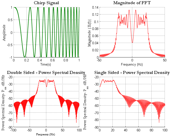
The following wrapper script utilizes the above function and generates a chirp with starting frequency $latex f_0=1Hz$ at the start of the time base and $latex f_1=25 Hz$ at $latex t_1=1s$ which is the end of the time base. From the PSD plot, it can be ascertained that the signal energy is concentrated only upto 25 Hz
fs=500; %sampling frequency
t=0:1/fs:1; %time base - upto 1 second

f0=1;% starting frequency of the chirp
f1=fs/20; %frequency of the chirp at t1=1 second
x = mychirp(t,f0,1,f1);
subplot(2,2,1)
plot(t,x,'k');
title(['Chirp Signal']);
xlabel('Time(s)');
ylabel('Amplitude');
FFT and power spectral density
As with other signals, describes in the previous posts, let’s plot the FFT of the generated chirp signal and its power spectral density (PSD).
L=length(x);
NFFT = 1024;
X = fftshift(fft(x,NFFT));
Pxx=X.*conj(X)/(NFFT*NFFT); %computing power with proper scaling
f = fs*(-NFFT/2:NFFT/2-1)/NFFT; %Frequency Vector

subplot(2,2,2)
plot(f,abs(X)/(L),'r');
title('Magnitude of FFT');
xlabel('Frequency (Hz)')
ylabel('Magnitude |X(f)|');
xlim([-50 50])


Pxx=X.*conj(X)/(NFFT*NFFT); %computing power with proper scaling
subplot(2,2,3)
plot(f,10*log10(Pxx),'r');
title('Double Sided - Power Spectral Density');
xlabel('Frequency (Hz)')
ylabel('Power Spectral Density- P_{xx} dB/Hz');
xlim([-100 100])

X = fft(x,NFFT);
X = X(1:NFFT/2+1);%Throw the samples after NFFT/2 for single sided plot
Pxx=X.*conj(X)/(NFFT*NFFT);
f = fs*(0:NFFT/2)/NFFT; %Frequency Vector
subplot(2,2,4)
plot(f,10*log10(Pxx),'r');
title('Single Sided - Power Spectral Density');
xlabel('Frequency (Hz)')
ylabel('Power Spectral Density- P_{xx} dB/Hz');
Rate this article: [ratings]
References:
[1] Patrick Flandrin,“Chirps everywhere”,CNRS — Ecole Normale Supérieure de Lyon
Does anyone know any way to produce a chirp in Matlab that follows a custom polynomial rather than the pre-built in functions provided in the chirp() function?
Does the chirp() function allow for more customization than I am aware of?
I want to produce a chirp based on the following polynomial (determined using polyfit() on a set of data points)…
y2 = p(1).*x.^10 + p(2).*x.^9 + p(3).*x.^8 + p(4).*x.^7 + p(5).*x.^6 + p(6).*x.^5 + p(7).*x.^4 + p(8).*x.^3 + p(9).*x.^2 + p(10).*x + p(11) ;
Please check the references below:
http://rfmw.em.keysight.com/wireless/helpfiles/n7620a/Content/Main/Polynomial_Chirp.htm
http://perso.ens-lyon.fr/patrick.flandrin/SPIE01_PF.pdf
Hi Mathuranathan. Thanks for the detailed explanation. Is there a typo? Formula (2) correctly states “x(t) = Acos(Ɵ(t))”. But immediately after that you state “where Ɵ(t) = ω0 + Ф is the instantaneous phase and it is linear in time.” Looks like there’s a ‘t’ missing: I think it should read “where Ɵ(t) = ω0t + Ф is the instantaneous phase and it is linear in time.”
Dear Lloyd,
Thanks for spotting the typo. It is corrected now.
Hey nice article. I have a question: why is the amplitude of the second plot (magnitude of fft) not one? Because all the frequencys in your chirp signal have the amplitude of one? Am I missing something
The frequency of the chirp signal varies with time, hence the amplitude of each frequency component does not stay the same. To have a same amplitude for all frequencies, the signal needs to have 1 complete cycle for each frequency component. For chirp, the frequency continuously changes from one time instant to the next, you cannot pin-point a cycle.
White noise is an excellent example that has a flat magnitude for all frequencies. See here: https://www.gaussianwaves.com/2013/11/simulation-and-analysis-of-white-noise-in-matlab/
Thank you Mathuranathan
My question could I multiply the the values of frequency (in second graph) by the ratio (1/0.1, which is the amplitude of of chirp signal on the amplitude of FFt), and then we have a frequency-acceleration graph?
Regards
The FFT graph for Chirp just shows the spectral content of the chirp signal at various frequencies. The values returned by FFT are just raw amplitude values.
Acceleration or velocities are measured in time domain, not in frequency domain. Hence, to plot frequency vs. acceleration, you need some kind of Frequency Response Function (FRF). Some examples here: http://www.vibrationdata.com/tutorials2/frf.pdf
In line 14 of the mychirp function, shouldn’t x be defined as x=cos(2pi(kt+f0).t+phase) instead?
It follows from equations (5) and (10). I have re-written that portion for clarity. Hope it helps.
I want to add into my question that there seems to be a difference between Eq(6) and Eq(8). Can you explain this difference?
Yes, they were different because of different assumption on omega_i(t). However, it is irrelevant to the derivation and hence it is removed in this re-edited article.
Hello Mathuranathan
Great article with proper detailed explanations about chirps! Regarding PSD, may I know why you have scaled the magnitude^2 by NFFT twice (psd = X.conj(X)/(NFFTNFFT))?
I obtained the denominator factor (NFFT*NFFT) from empirical result. In the following page I have explained how the total power of a sinusoidal signal can calculated from the signal samples in time-domain and verified it against frequency domain calculation.
https://www.gaussianwaves.com/2013/12/computation-of-power-of-a-signal-in-matlab-simulation-and-verification/
Thank you very much for redirecting to the other article, Mathuranathan! That plus this youtube video (https://www.youtube.com/watch?v=D67ZgH8FEAI) helped me understand the concept of PSD much better!
Hello Mathuranathan
plot(f,abs(X)/(L),’r’);
Why abs(X) is divide by (L)? Can’t we just write plot(f,abs(X),’r’); only?
Thank You.
FFT is taken on a vector of size L. Hence the amplitude is normalized by dividing by L. If the shape of the amplitude spectrum is important than the actual amplitude values, then the scaling factor can be ignored.
Hello Mathuranathan
Can you plz explain
What is difference between normal sinusoidal or chrip signal ?
Sinusoidal signal is a smooth repetition of oscillation at a fixed frequency. Chirp signal is also a sinusoidal signal whose frequency continuously increases (or decreases).
what is the physical significance of Magnitude response?
Magnitude response is the magnitude of the complex value of the frequency response vs. frequency.
It is used to see how a system affects the amplitudes of frequencies in a signal.
A variable’s amplitude is just a measure of change relative to its central position, whereas a variable’s magnitude is a measure of distance or quantity regardless of direction.
What does PSD of chirp signals tells us? What can we comment on the PSD graph of chirp signal?
The power spectral density tell us the distribution of power of the signal vs. frequency. The PSD plots indicate most of the power is concentrated from 1Hz to 25 Hz which conforms with the intended configuration of the chirp in the time domain.
Sir can you tell a bit more difference between normal sinusoidal vs chirp signal.
(Atleast 5 difference)