Synopsis: Cyclic prefix in OFDM, tricks a natural channel to perform circular convolution. This simplifies equalizer design at the receiver. Hands-on demo in Matlab.
Cyclic Prefix-ed OFDM
A cyclic-prefixed OFDM (CP-OFDM) transceiver architecture is typically implemented using inverse discrete Fourier transform (IDFT) and discrete Fourier transform (DFT) blocks (refer Figure 13.3). In an OFDM transmitter, the modulated symbols are assigned to individual subcarriers and sent to an IDFT block. The output of the IDFT block, generally viewed as time domain samples, results in an OFDM symbol. Such OFDM symbols are then transmitted across a channel with certain channel impulse response (CIR). On the other hand, the receiver applies DFT over the received OFDM symbols for further demodulation of the information in the individual subcarriers.
This article is part of the book |
In reality, a multipath channel or any channel in nature acts as a linear filter on the transmitted OFDM symbols. Mathematically, the transmitted OFDM symbol (denoted as

![s[n]](https://s0.wp.com/latex.php?latex=s%5Bn%5D&bg=ffffff&fg=000&s=0&c=20201002)

![h[n]](https://s0.wp.com/latex.php?latex=h%5Bn%5D&bg=ffffff&fg=000&s=0&c=20201002)

![w[n]](https://s0.wp.com/latex.php?latex=w%5Bn%5D&bg=ffffff&fg=000&s=0&c=20201002)


![r[n] = h[n] \ast s[n] + w[n] \;\;\; (\ast \rightarrow linear\;convolution ) \quad\quad (1)](https://s0.wp.com/latex.php?latex=r%5Bn%5D+%3D+h%5Bn%5D+%5Cast+s%5Bn%5D+%2B+w%5Bn%5D+%5C%3B%5C%3B%5C%3B+%28%5Cast+%5Crightarrow+linear%5C%3Bconvolution+%29+%5Cquad%5Cquad+%281%29+&bg=ffffff&fg=000&s=2&c=20201002)
The idea behind using OFDM is to combat frequency selective fading, where different frequency components of a transmitted signal can undergo different levels of fading. The OFDM divides the available spectrum in to small chunks called sub-channels. Within the subchannels, the fading experienced by the individual modulated symbol can be considered flat. This opens-up the possibility of using a simple frequency domain equalizer to neutralize the channel effects in the individual subchannels.
Circular convolution and designing a simple frequency domain equalizer
From one of the DFT properties, we know that the circular convolution of two sequences in time domain is equivalent to the multiplication of their individual responses in frequency domain.
Let


![S[k]](https://s0.wp.com/latex.php?latex=S%5Bk%5D&bg=ffffff&fg=000&s=0&c=20201002)

![H[k]](https://s0.wp.com/latex.php?latex=H%5Bk%5D&bg=ffffff&fg=000&s=0&c=20201002)


![h[n] \circledast s[n] \equiv H[k] S[k] \quad\quad (2)](https://s0.wp.com/latex.php?latex=h%5Bn%5D+%5Ccircledast+s%5Bn%5D+%5Cequiv+H%5Bk%5D+S%5Bk%5D+%5Cquad%5Cquad+%282%29+&bg=ffffff&fg=000&s=2&c=20201002)
If we ignore channel noise in the OFDM transmission, the received signal is written as

![r[n] = h[n] \ast s[n] \quad\quad (\ast \rightarrow linear\;convolution ) \quad\quad (3)](https://s0.wp.com/latex.php?latex=r%5Bn%5D+%3D+h%5Bn%5D+%5Cast+s%5Bn%5D+%5Cquad%5Cquad+%28%5Cast+%5Crightarrow+linear%5C%3Bconvolution+%29+%5Cquad%5Cquad+%283%29+&bg=ffffff&fg=000&s=2&c=20201002)
We can note that the channel performs a linear convolution operation on the transmitted signal. Instead, if the channel performs circular convolution (which is not the case in nature) then the equation would have been

![r[n] = h[n] \circledast s[n] \quad\quad (\circledast \rightarrow circular\;convolution ) \quad\quad (4)](https://s0.wp.com/latex.php?latex=r%5Bn%5D+%3D+h%5Bn%5D+%5Ccircledast+s%5Bn%5D+%5Cquad%5Cquad+%28%5Ccircledast+%5Crightarrow+circular%5C%3Bconvolution+%29+%5Cquad%5Cquad+%284%29+&bg=ffffff&fg=000&s=2&c=20201002)
By applying the DFT property given in equation 2,

![r[n] = h[n] \circledast s[n] \quad\quad \equiv R[k] = H[k] S[k] \quad\quad (5)](https://s0.wp.com/latex.php?latex=r%5Bn%5D+%3D+h%5Bn%5D+%5Ccircledast+s%5Bn%5D+%5Cquad%5Cquad+%5Cequiv+R%5Bk%5D+%3D+H%5Bk%5D+S%5Bk%5D+%5Cquad%5Cquad+%285%29+&bg=ffffff&fg=000&s=2&c=20201002)
As a consequence, the channel effects can be neutralized at the receiver using a simple frequency domain equalizer (actually this is a zero-forcing equalizer when viewed in time domain) that just inverts the estimated channel response and multiplies it with the frequency response of the received signal to obtain the estimates of the OFDM symbols in the subcarriers as

![\hat{S}[k] = \frac{R[k]}{H[k]} \quad\quad (6)](https://s0.wp.com/latex.php?latex=%5Chat%7BS%7D%5Bk%5D+%3D+%5Cfrac%7BR%5Bk%5D%7D%7BH%5Bk%5D%7D+%5Cquad%5Cquad+%286%29+&bg=ffffff&fg=000&s=2&c=20201002)
Demonstrating the role of Cyclic Prefix
The simple frequency domain equalizer shown in equation 6 is possible only if the channel performs circular convolution. But in nature, all channels perform linear convolution. The linear convolution can be converted into circular convolution by adding Cyclic Prefix (CP) in the OFDM architecture. The addition of CP makes the linear convolution imparted by the channel appear as circular convolution to the DFT process at the receiver (Reference [1]).
Let’s understand this by demonstration.
To simply stuffs, we will create two randomized vectors for


N=8; %period of DFT
s = randn(1,8);
h = randn(1,3);
>> s =   -0.0155    2.5770    1.9238   -0.0629   -0.8105    0.6727   -1.5924   -0.8007
>> h =   -0.4878   -1.5351    0.2355
Now, convolve the vectors


lin_s_h = conv(h,s) %linear convolution of h and s
cir_s_h = cconv(h,s,N) % circular convolution of h and s with period N
lin_s_h = 0.0076 -1.2332 -4.8981 -2.3158  0.9449  0.9013 -0.4468  2.9934  0.8542 -0.1885
cir_s_h = 0.8618 -1.4217 -4.8981 -2.3158  0.9449  0.9013 -0.4468  2.9934


Let’s append a cyclic prefix to the signal


Ncp = 2; %number of symbols to copy and paste for CP
s_cp = [s(end-Ncp+1:end) s]; %copy last Ncp symbols from s and prefix it.
s_cp = -1.5924 -0.8007 -0.0155 2.5770 1.9238 -0.0629 -0.8105 0.6727 -1.5924 -0.8007
Lets assume that we send the cyclic-prefixed OFDM symbol


lin_scp_h = conv(h,s_cp) %linear convolution of CP-OFDM symbol s_cp and the CIR h
lin_scp_h = 0.7767 2.8350 0.8618 -1.4217 -4.8981 -2.3158 0.9449 0.9013 -0.4468 2.9934 0.8542 -0.1885
Compare the outputs due to cir_s_h


cir_s_h   = 0.8618  -1.4217 -4.8981 -2.3158  0.9449  0.9013 -0.4468  2.9934
lin_scp_h = 0.7767   2.8350  0.8618 -1.4217 -4.8981 -2.3158  0.9449  0.9013 -0.4468 2.9934 0.8542 -0.1885
We have just tricked the channel to perform circular convolution by adding a cyclic extension to the OFDM symbol. At the receiver, we are only interested in the middle section of the lin_scp_h which is the channel output. The first block in the OFDM receiver removes the additional symbols from the front and back of the channel output. The resultant vector is the received symbol r after the removal of cyclic prefix in the receiver.
r = lin_scp_h(Ncp+1:N+Ncp)%cut from index Ncp+1 to N+Ncp
Verifying DFT property
The DFT property given in equation 5 can be re-written as


To verify this in Matlab, take N-point DFTs of the received signal and CIR. Then, we can see that the IDFT of product of DFTs of
R = fft(r,N); %frequency response of received signal
H = fft(h,N); %frequency response of CIR
S = fft(s,N); %frequency response of OFDM signal (non CP)

r1 = ifft(S.*H); %IFFT of product of individual DFTs

display(['IFFT(DFT(H)*DFT(S)) : ',num2str(r1)])
display([cconv(s,h): ', numstr(r)])
IFFT(DFT(H)*DFT(S)) : 0.86175  -1.4217  -4.8981  -2.3158  0.94491  0.90128 -0.44682  2.9934
cconv(s,h):           0.86175  -1.4217  -4.8981  -2.3158  0.94491  0.90128 -0.44682  2.9934
Rate this article: Note: There is a rating embedded within this post, please visit this post to rate it.
Reference:
Topics in this chapter
| Orthogonal Frequency Division Multiplexing (OFDM) ● Introduction ● Understanding the role of cyclic prefix in a CP-OFDM system □ Circular convolution and designing a simple frequency domain equalizer □ Demonstrating the role of cyclic prefix □ Verifying DFT property ● Discrete-time implementation of baseband CP-OFDM ● Performance of MPSK-CP-OFDM and MQAM-CP-OFDM on AWGN channel ● Performance of MPSK-CP-OFDM and MQAM-CP-OFDM on frequency selective Rayleigh channel |
Books by the author
 Wireless Communication Systems in Matlab Second Edition(PDF) |  Digital Modulations using Python (PDF ebook) |  Digital Modulations using Matlab (PDF ebook) |
| Hand-picked Best books on Communication Engineering Best books on Signal Processing |
||


![a=[a_0,a_1,a_2,...,a_{n-1}]](https://s0.wp.com/latex.php?latex=a%3D%5Ba_0%2Ca_1%2Ca_2%2C...%2Ca_%7Bn-1%7D%5D&bg=ffffff&fg=000&s=0&c=20201002)

![a=[a_0,a_1,a_2,...,a_n]](https://s0.wp.com/latex.php?latex=a%3D%5Ba_0%2Ca_1%2Ca_2%2C...%2Ca_n%5D&bg=ffffff&fg=000&s=0&c=20201002)

![b=[b_0,b_1,b_2,...,b_n]](https://s0.wp.com/latex.php?latex=b%3D%5Bb_0%2Cb_1%2Cb_2%2C...%2Cb_n%5D&bg=ffffff&fg=000&s=0&c=20201002)


![p(x) . q(x)=(p\ast q)(x)=a.b=[c_0,c_1,c_2,\cdots,c_{n+m}] \; , \;where](https://s0.wp.com/latex.php?latex=p%28x%29+.+q%28x%29%3D%28p%5Cast+q%29%28x%29%3Da.b%3D%5Bc_0%2Cc_1%2Cc_2%2C%5Ccdots%2Cc_%7Bn%2Bm%7D%5D+%5C%3B+%2C+%5C%3Bwhere+&bg=ffffff&fg=000&s=2&c=20201002)


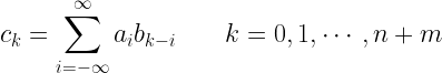

![c[k]=\displaystyle{\sum_{i=-\infty}^{\infty}a[i]b[k-i]} \quad\quad k=0,1,\cdots,n+m](https://s0.wp.com/latex.php?latex=c%5Bk%5D%3D%5Cdisplaystyle%7B%5Csum_%7Bi%3D-%5Cinfty%7D%5E%7B%5Cinfty%7Da%5Bi%5Db%5Bk-i%5D%7D+%5Cquad%5Cquad+k%3D0%2C1%2C%5Ccdots%2Cn%2Bm+&bg=ffffff&fg=000&s=2&c=20201002)


![x[n]](https://s0.wp.com/latex.php?latex=x%5Bn%5D&bg=ffffff&fg=000&s=0&c=20201002)
![y[n]](https://s0.wp.com/latex.php?latex=y%5Bn%5D&bg=ffffff&fg=000&s=0&c=20201002)

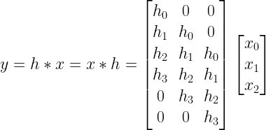
![y[k]=h[n]*x[n] = \displaystyle{\sum_{i=-\infty}^{\infty}x[i]h[k-i]}](https://s0.wp.com/latex.php?latex=y%5Bk%5D%3Dh%5Bn%5D%2Ax%5Bn%5D+%3D+%5Cdisplaystyle%7B%5Csum_%7Bi%3D-%5Cinfty%7D%5E%7B%5Cinfty%7Dx%5Bi%5Dh%5Bk-i%5D%7D+&bg=ffffff&fg=000&s=2&c=20201002)

![h[n]=[h_0,h_1,h_2,h_3]](https://s0.wp.com/latex.php?latex=h%5Bn%5D%3D%5Bh_0%2Ch_1%2Ch_2%2Ch_3%5D&bg=ffffff&fg=000&s=0&c=20201002)

![x[n]=[x_0,x_1,x_2]](https://s0.wp.com/latex.php?latex=x%5Bn%5D%3D%5Bx_0%2Cx_1%2Cx_2%5D&bg=ffffff&fg=000&s=0&c=20201002)

![h[n] \ast x[n]](https://s0.wp.com/latex.php?latex=h%5Bn%5D+%5Cast+x%5Bn%5D&bg=ffffff&fg=000&s=0&c=20201002)

![y[k]=h[n]*x[n] = \displaystyle{\sum_{i=-\infty}^{\infty}x[i]h[k-i]} \quad k=0,1,\cdots,5](https://s0.wp.com/latex.php?latex=y%5Bk%5D%3Dh%5Bn%5D%2Ax%5Bn%5D+%3D+%5Cdisplaystyle%7B%5Csum_%7Bi%3D-%5Cinfty%7D%5E%7B%5Cinfty%7Dx%5Bi%5Dh%5Bk-i%5D%7D+%5Cquad+k%3D0%2C1%2C%5Ccdots%2C5+&bg=ffffff&fg=000&s=2&c=20201002)


![\begin{bmatrix} y[0]\\y[1]\\y[2]\\y[3]\\y[4]\\y[5] \end{bmatrix}=\begin{bmatrix}h[0] &0 & 0 \\ h[1] & h[0] & 0 \\ h[2] & h[1] & h[0] \\ h[3] & h[2] & h[1] \\ 0 & h[3] & h[2] \\ 0 & 0 & h[3] \end{bmatrix} \begin{bmatrix}x[0]\\x[1]\\x[2] \end{bmatrix}](https://s0.wp.com/latex.php?latex=%5Cbegin%7Bbmatrix%7D+y%5B0%5D%5C%5Cy%5B1%5D%5C%5Cy%5B2%5D%5C%5Cy%5B3%5D%5C%5Cy%5B4%5D%5C%5Cy%5B5%5D+%5Cend%7Bbmatrix%7D%3D%5Cbegin%7Bbmatrix%7Dh%5B0%5D+%260+%26+0+%5C%5C+h%5B1%5D+%26+h%5B0%5D+%26+0+%5C%5C+h%5B2%5D+%26+h%5B1%5D+%26+h%5B0%5D+%5C%5C+h%5B3%5D+%26+h%5B2%5D+%26+h%5B1%5D+%5C%5C+0+%26+h%5B3%5D+%26+h%5B2%5D+%5C%5C+0+%26+0+%26+h%5B3%5D+%5Cend%7Bbmatrix%7D+%5Cbegin%7Bbmatrix%7Dx%5B0%5D%5C%5Cx%5B1%5D%5C%5Cx%5B2%5D+%5Cend%7Bbmatrix%7D+&bg=ffffff&fg=000&s=2&c=20201002)