Tag: GSM

Key focus: Know how to generate a gaussian pulse, compute its Fourier Transform using FFT and power spectral density (PSD) in Matlab & Python.

Numerous texts are available to explain the basics of Discrete Fourier Transform and its very efficient implementation – Fast Fourier Transform (FFT).  Often we are confronted with the need to generate simple, standard signals (sine, cosine, Gaussian pulse, squarewave, isolated rectangular pulse, exponential decay, chirp signal) for simulation purpose. I intend to show (in a series of articles) how these basic signals can be generated in Matlab and how to represent them in frequency domain using FFT.

This article is part of the following books ● Digital Modulations using Matlab : Build Simulation Models from Scratch, ISBN: 978-1521493885 ● Digital Modulations using Python ISBN: 978-1712321638 ● Wireless communication systems in Matlab ISBN: 979-8648350779 All books available in ebook (PDF) and Paperback formats

Gaussian Pulse : Mathematical description:

In digital communications, Gaussian Filters are employed in Gaussian Minimum Shift Keying – GMSK (used in GSM technology) and Gaussian Frequency Shift Keying (GFSK). Two dimensional Gaussian Filters are used in Image processing to produce Gaussian blurs. The impulse response of a Gaussian Filter is Gaussian. Gaussian Filters give no overshoot with minimal rise and fall time when excited with a step function. Gaussian Filter has minimum group delay. The impulse response of a Gaussian Filter is written as a Gaussian Function as follows

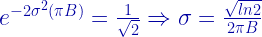
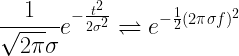
The Fourier Transform of a Gaussian pulse preserves its shape.

The above derivation makes use of the following result from complex analysis theory and the property of Gaussian function – total area under Gaussian function integrates to 1.

By change of variable, let ( ). 

Thus, the Fourier Transform of a Gaussian pulse is a Gaussian Pulse.

Gaussian Pulse – Fourier Transform using FFT (Matlab & Python):

The following code generates a Gaussian Pulse with ( ). The Discrete Fourier Transform of this digitized version of Gaussian Pulse is plotted with the help of (FFT) function in Matlab.

For Python code, please refer the book Digital Modulations using Python

fs=80; %sampling frequency
sigma=0.1;
t=-0.5:1/fs:0.5; %time base

variance=sigma^2;
x=1/(sqrt(2*pi*variance))*(exp(-t.^2/(2*variance)));
subplot(2,1,1)
plot(t,x,'b');
title(['Gaussian Pulse \sigma=', num2str(sigma),'s']);
xlabel('Time(s)');
ylabel('Amplitude');

L=length(x);
NFFT = 1024;
X = fftshift(fft(x,NFFT));
Pxx=X.*conj(X)/(NFFT*NFFT); %computing power with proper scaling
f = fs*(-NFFT/2:NFFT/2-1)/NFFT; %Frequency Vector

subplot(2,1,2)
plot(f,abs(X)/fs,'r');
title('Magnitude of FFT');
xlabel('Frequency (Hz)')
ylabel('Magnitude |X(f)|');
xlim([-10 10])

Double Sided and Single Power Spectral Density using FFT:

Next, the Power Spectral Density (PSD) of the Gaussian pulse is constructed using the FFT. PSD describes the power contained at each frequency component of the given signal. Double Sided power spectral density is plotted first, followed by single sided power spectral density plot (retaining only the positive frequency side of the spectrum).

Pxx=X.*conj(X)/(L*L); %computing power with proper scaling
figure;
plot(f,10*log10(Pxx),'r');
title('Double Sided - Power Spectral Density');
xlabel('Frequency (Hz)')
ylabel('Power Spectral Density- P_{xx} dB/Hz');

X = fft(x,NFFT);
X = X(1:NFFT/2+1);%Throw the samples after NFFT/2 for single sided plot
Pxx=X.*conj(X)/(L*L);
f = fs*(0:NFFT/2)/NFFT; %Frequency Vector
figure;
plot(f,10*log10(Pxx),'r');
title('Single Sided - Power Spectral Density');
xlabel('Frequency (Hz)')
ylabel('Power Spectral Density- P_{xx} dB/Hz');

For Python code, please refer the book Digital Modulations using Python

Rate this article: Note: There is a rating embedded within this post, please visit this post to rate it.

Topics in this chapter

Essentials of Signal Processing ● Generating standard test signals  □ Sinusoidal signals  □ Square wave  □ Rectangular pulse  □ Gaussian pulse  □ Chirp signal ● Interpreting FFT results - complex DFT, frequency bins and FFTShift  □ Real and complex DFT  □ Fast Fourier Transform (FFT)  □ Interpreting the FFT results  □ FFTShift  □ IFFTShift ● Obtaining magnitude and phase information from FFT  □ Discrete-time domain representation  □ Representing the signal in frequency domain using FFT  □ Reconstructing the time domain signal from the frequency domain samples ● Power spectral density ● Power and energy of a signal  □ Energy of a signal  □ Power of a signal  □ Classification of signals  □ Computation of power of a signal - simulation and verification ● Polynomials, convolution and Toeplitz matrices  □ Polynomial functions  □ Representing single variable polynomial functions  □ Multiplication of polynomials and linear convolution  □ Toeplitz matrix and convolution ● Methods to compute convolution  □ Method 1: Brute-force method  □ Method 2: Using Toeplitz matrix  □ Method 3: Using FFT to compute convolution  □ Miscellaneous methods ● Analytic signal and its applications  □ Analytic signal and Fourier transform  □ Extracting instantaneous amplitude, phase, frequency  □ Phase demodulation using Hilbert transform ● Choosing a filter : FIR or IIR : understanding the design perspective  □ Design specification  □ General considerations in design

Books by the author

Wireless Communication Systems in Matlab Second Edition(PDF) Note: There is a rating embedded within this post, please visit this post to rate it. $14.99 – Add to Cart Checkout Added to cart	Digital Modulations using Python (PDF ebook) Note: There is a rating embedded within this post, please visit this post to rate it. $14.99 – Add to Cart Checkout Added to cart	Digital Modulations using Matlab (PDF ebook) Note: There is a rating embedded within this post, please visit this post to rate it. $14.99 – Add to Cart Checkout Added to cart
Hand-picked Best books on Communication Engineering Best books on Signal Processing