The Shannon power efficiency limit is the limit of a band-limited system irrespective of modulation or coding scheme. It informs us the minimum required energy per bit required at the transmitter for reliable communication. It is also called unconstrained Shannon power efficiency Limit. If we select a particular modulation scheme or an encoding scheme, we calculate the constrained Shannon limit for that scheme.
One of the objective of a communication system design is to reliably send information at the lowest possible power level. The system should be able to provide acceptable bit-error-rate (BER) performance at the lowest possible power level. Often, this performance is charted in terms of BER Vs. . The quantity is called power efficiency, denoted as . Power efficiency is defined as the ratio of signal energy per bit () to noise power spectral density per bit ( – required at the receiver input to achieve certain BER.
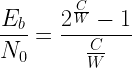
Re-writing in terms of spectral efficiency , the Shannon limit on power efficiency for reliable communication is given by
With this equation, we can calculate the minimum required to achieve a certain spectral efficiency. As an example, lets simulate and plot the relationship between and spectral efficiency , as given in equation (3).
k =0.1:0.001:15; EbN0=(2.ˆk-1)./k;
semilogy(10*log10(EbN0),k);
xlabel('E_b/N_o (dB)');ylabel('Spectral Efficiency (\eta)');
title('Channel Capacity & Power efficiency limit')
hold on;grid on; xlim([-2 20]);ylim([0.1 10]);
yL = get(gca,'YLim');
line([-1.59 -1.59],yL,'Color','r','LineStyle','--');
The ultimate Shannon limit
From the plot in Fig. 1, we notice that the Shannon limit on is a monotonic function of . When , the Shannon limit on is equal to . If , the limit is at . When , the Shannon limit on approaches . This value is called ultimate Shannon limit or specifically absolute Shannon power efficiency limit. This limit informs us the minimum required energy per bit required at the transmitter for reliable communication. It is one among the important measures in designing a coding scheme.
Figure 1: Shannon Power Efficiency Limit
The ultimate Shannon limit can be derived using L’Hospital’s rule as follows. The asymptotic value, , that we are seeking, is the value of as the spectral efficiency approaches .
Let and . As and the argument of the limit becomes indeterminate (), L’Hospital’s rule can be applied in this case. According to L’Hospital’s rule, if and are both zero or are both , then for any value of .
Thus, the next step boils down to finding the first derivative of and . Expressing in natural logarithm.
Let and , then by chain rule of differentiation,
Since , the first derivative of is
Using equations (8) and (9), and applying L’Hospital’s rule, the Shannon’s limit on is given by
The absolute Shannon power efficiency limit is the limit of a band-limited system irrespective of modulation or coding scheme. This is also called unconstrained Shannon power efficiency Limit. If we select a particular modulation scheme or an encoding scheme, we calculate the constrained Shannon limit for that scheme.
Shannon power efficiency limit does not depend on error probability. Shannon limit tells us the minimum possible required for achieving an arbitrarily small probability of error as , where is the number of signaling levels for the modulation technique, for BPSK , QPSK and so on. It gives the minimum possible that satisfies the Shannon theorem. In other words, it gives the minimum possible required to achieve maximum transmission capacity ( , where, is the rate of transmission and is the channel capacity). It will not specify error probability at that limit. Nor will it give any direction on coding technique that can be used to achieve that limit. As the capacity is approached, the system complexity will increase drastically. So the aim of any system design is to achieve that limit. For example, the error probability performances of Turbo codes are very close to Shannon limit [1].
As an example, let’s evaluate the performance of a 2-PAM (Pulse Amplitude Modulation) system and determine the maximum possible coding gain that can be achieved by the most advanced coding scheme. The methodology for simulating the performance of a 2-PAM system is described in chapter 5 and 6. Using this methodology, the performance of a 2-PAM system is simulated and plotted in Figure 2. The absolute Shannon power efficiency limits when the spectral efficiency is and are also referenced on the plot.
The spectral efficiency of an ideal 2-PAM system is . Hence, if the target bit error rate is , then a coding gain of can be achieved using powerful codes, if we have to maintain the nominal spectral efficiency at .
If there is no limit on the spectral efficiency, then we can let . In this case, the absolute Shannon power efficiency limit is when . Thus a coding gain of approximately is possible with powerful codes if we let the spectral efficiency approach zero.
Rate this article: Note: There is a rating embedded within this post, please visit this post to rate it.
Key focus: Compare Performance and spectral efficiency of bandwidth-efficient digital modulation techniques (BPSK,QPSK and QAM) on their theoretical BER over AWGN.
Let’s take up some bandwidth-efficient linear digital modulation techniques (BPSK,QPSK and QAM) and compare its performance based on their theoretical BER over AWGN. (Readers are encouraged to read previous article on Shannon’s theorem and channel capacity).
Table 1 summarizes the theoretical BER (given SNR per bit ration – Eb/N0) for various linear modulations. Note that the Eb/N0 values used in that table are in linear scale [to convert Eb/N0 in dB to linear scale – use Eb/N0(linear) = 10^(Eb/N0(dB)/10) ]. A small script written in Matlab (given below) gives the following output.
Figure 1: Eb/N0 Vs. BER for various digital modulations over AWGN channel
Table 1: Theoretical BER over AWGN for various linear digital modulation techniques
The following table is obtained by extracting the values of Eb/N0 to achieve BER=10-6 from Figure-1. (Table data sorted with increasing values of Eb/N0).
Table 2: Capacity of various modulations their efficiency and channel bandwidth
where,
is the bandwidth efficiency for linear modulation with M point constellation, meaning that ηBbits can be stuffed in one symbol with Rb bits/sec data rate for a given minimum bandwidth.
is the minimum bandwidth needed for information rate of Rb bits/second. If a pulse shaping technique like raised cosine pulse [with roll off factor (a)] is used then Bmin becomes
Next the data in table 2 is plotted with Eb/N0 on the x-axis and ηon the y-axis (see figure 2) along with the well known Shannon’s Capacity equation over AWGN given by,
which can be represented as (refer [1])
Figure 2: Spectral efficiency vs Eb/N0 for various modulations at Pb=10-6
Rate this article: Note: There is a rating embedded within this post, please visit this post to rate it.
Matlab Code
EbN0dB=-4:1:24;
EbN0lin=10.^(EbN0dB/10);
colors={'b-*','g-o','r-h','c-s','m-d','y-*','k-p','b-->','g:<','r-.d'};
index=1;

%BPSK
BPSK = 0.5*erfc(sqrt(EbN0lin));
plotHandle=plot(EbN0dB,log10(BPSK),char(colors(index)));
set(plotHandle,'LineWidth',1.5);
hold on;

index=index+1;

%M-PSK
m=2:1:5;
M=2.^m;
for i=M,
    k=log2(i);
    berErr = 1/k*erfc(sqrt(EbN0lin*k)*sin(pi/i));
    plotHandle=plot(EbN0dB,log10(berErr),char(colors(index)));
    set(plotHandle,'LineWidth',1.5);
    index=index+1;
end

%Binary DPSK
Pb = 0.5*exp(-EbN0lin);
plotHandle = plot(EbN0dB,log10(Pb),char(colors(index)));
set(plotHandle,'LineWidth',1.5);
index=index+1;

%Differential QPSK
a=sqrt(2*EbN0lin*(1-sqrt(1/2)));
b=sqrt(2*EbN0lin*(1+sqrt(1/2)));
Pb = marcumq(a,b,1)-1/2.*besseli(0,a.*b).*exp(-1/2*(a.^2+b.^2));
plotHandle = plot(EbN0dB,log10(Pb),char(colors(index)));
set(plotHandle,'LineWidth',1.5);
index=index+1;

%M-QAM
m=2:2:6;
M=2.^m;

for i=M,
    k=log2(i);
    berErr = 2/k*(1-1/sqrt(i))*erfc(sqrt(3*EbN0lin*k/(2*(i-1))));
    plotHandle=plot(EbN0dB,log10(berErr),char(colors(index)));
    set(plotHandle,'LineWidth',1.5);
    index=index+1;
end

legend('BPSK','QPSK','8-PSK','16-PSK','32-PSK','D-BPSK','D-QPSK','4-QAM','16-QAM','64-QAM');
axis([-4 24 -8 0]);
set(gca,'XTick',-4:2:24); %re-name axis accordingly
ylabel('Probability of BER Error - log10(Pb)');
xlabel('Eb/N0 (dB)');
title('Probability of BER Error log10(Pb) Vs Eb/N0');
grid on;
Shannon theorem dictates the maximum data rate at which the information can be transmitted over a noisy band-limited channel. The maximum data rate is designated as channel capacity. The concept of channel capacity is discussed first, followed by an in-depth treatment of Shannon’s capacity for various channels.
Introduction
The main goal of a communication system design is to satisfy one or more of the following objectives.
● The transmitted signal should occupy smallest bandwidth in the allocated spectrum – measured in terms of bandwidth efficiency also called as spectral efficiency – \(\eta_B\). ● The designed system should be able to reliably send information at the lowest practical power level. This is measured in terms of power efficiency – \(\eta_P\). ● Ability to transfer data at higher rates – \(R\) bits=second. ● The designed system should be robust to multipath effects and fading. ● The system should guard against interference from other sources operating in the same frequency – low carrier-to-cochannel signal interference ratio (CCI). ● Low adjacent channel interference from near by channels – measured in terms of adjacent channel Power ratio (ACPR). ● Easier to implement and lower operational costs.
Chapter 2 in my book ‘Wireless Communication systems in Matlab’, is intended to describe the effect of first three objectives when designing a communication system for a given channel. A great deal of information about these three factors can be obtained from Shannon’s noisy channel coding theorem.
Shannon’s noisy channel coding theorem
For any communication over a wireless link, one must ask the following fundamental question: What is the optimal performance achievable for a given channel ?. The performance over a communication link is measured in terms of capacity, which is defined as the maximum rate at which the information can be transmitted over the channel with arbitrarily small amount of error.
It was widely believed that the only way for reliable communication over a noisy channel is to reduce the error probability as small as possible, which in turn is achieved by reducing the data rate. This belief was changed in 1948 with the advent of Information theory by Claude E. Shannon. Shannon showed that it is in fact possible to communicate at a positive rate and at the same time maintain a low error probability as desired. However, the rate is limited by a maximum rate called the channel capacity. If one attempts to send data at rates above the channel capacity, it will be impossible to recover it from errors. This is called Shannon’s noisy channel coding theorem and it can be summarized as follows:
● A given communication system has a maximum rate of information – C, known as the channel capacity. ● If the transmission information rate R is less than C, then the data transmission in the presence of noise can be made to happen with arbitrarily small error probabilities by using intelligent coding techniques. ● To get lower error probabilities, the encoder has to work on longer blocks of signal data. This entails longer delays and higher computational requirements.
The theorem indicates that with sufficiently advanced coding techniques, transmission that nears the maximum channel capacity – is possible with arbitrarily small errors. One can intuitively reason that, for a given communication system, as the information rate increases, the number of errors per second will also increase.
Shannon’s noisy channel coding theorem is a generic framework that can be applied to specific scenarios of communication. For example, communication through a band-limited channel in presence of noise is a basic scenario one wishes to study. Therefore, study of information capacity over an AWGN (additive white gaussian noise) channel provides vital insights, to the study of capacity of other types of wireless links, like fading channels.
Unconstrained capacity for band-limited AWGN channel
Real world channels are essentially continuous in both time as well as in signal space. Real physical channels have two fundamental limitations : they have limited bandwidth and the power/energy of the input signal to such channels is also limited. Therefore, the application of information theory on such continuous channels should take these physical limitations into account. This will enable us to exploit such continuous channels for transmission of discrete information.
In this section, the focus is on a band-limited real AWGN channel, where the channel input and output are real and continuous in time. The capacity of a continuous AWGN channel that is bandwidth limited to \(B\) Hz and average received power constrained to \(P\) Watts, is given by
Here, \(N_0/2\) is the power spectral density of the additive white Gaussian noise and \(P\) is the average power given by
\[P = E_b R \quad \quad (2) \]
where \(E_b\) is the average signal energy per information bit and \(R\) is the data transmission rate in bits-per-second. The ratio \(P/(N_0B)\) is the signal to noise ratio (SNR) per degree of freedom. Hence, the equation can be re-written as
Here, \(C\) is the maximum capacity of the channel in bits/second. It is also called Shannon’s capacity limit for the given channel. It is the fundamental maximum transmission capacity that can be achieved using the basic resources available in the channel, without going into details of coding scheme or modulation. It is the best performance limit that we hope to achieve for that channel. The above expression for the channel capacity makes intuitive sense:
● Bandwidth limits how fast the information symbols can be sent over the given channel. ● The SNR ratio limits how much information we can squeeze in each transmitted symbols. Increasing SNR makes the transmitted symbols more robust against noise. SNR represents the signal quality at the receiver front end and it depends on input signal power and the noise characteristics of the channel. ● To increase the information rate, the signal-to-noise ratio and the allocated bandwidth have to be traded against each other. ● For a channel without noise, the signal to noise ratio becomes infinite and so an infinite information rate is possible at a very small bandwidth. ● We may trade off bandwidth for SNR. However, as the bandwidth B tends to infinity, the channel capacity does not become infinite – since with an increase in bandwidth, the noise power also increases.
The Shannon’s equation relies on two important concepts: ● That, in principle, a trade-off between SNR and bandwidth is possible ● That, the information capacity depends on both SNR and bandwidth
It is worth to mention two important works by eminent scientists prior to Shannon’s paper [1]. Edward Amstrong’s earlier work on Frequency Modulation (FM) is an excellent proof for showing that SNR and bandwidth can be traded off against each other. He demonstrated in 1936, that it was possible to increase the SNR of a communication system by using FM at the expense of allocating more bandwidth [2]
In 1903, W.M Miner in his patent (U. S. Patent 745,734 [3]), introduced the concept of increasing the capacity of transmission lines by using sampling and time division multiplexing techniques. In 1937, A.H Reeves in his French patent (French Patent 852,183, U.S Patent 2,272,070 [4]) extended the system by incorporating a quantizer, there by paving the way for the well-known technique of Pulse Coded Modulation (PCM). He realized that he would require more bandwidth than the traditional transmission methods and used additional repeaters at suitable intervals to combat the transmission noise. With the goal of minimizing the quantization noise, he used a quantizer with a large number of quantization levels. Reeves patent relies on two important facts:
● One can represent an analog signal (like speech) with arbitrary accuracy, by using sufficient frequency sampling, and quantizing each sample in to one of the sufficiently large pre-determined amplitude levels ● If the SNR is sufficiently large, then the quantized samples can be transmitted with arbitrarily small errors
It is implicit from Reeve’s patent – that an infinite amount of information can be transmitted on a noise free channel of arbitrarily small bandwidth. This links the information rate with SNR and bandwidth.
Please refer [1] and [5] for the actual proof by Shannon. A much simpler version of proof (I would rather call it an illustration) can be found at [6].
This website uses cookies to improve your experience while you navigate through the website. Out of these, the cookies that are categorized as necessary are stored on your browser as they are essential for the working of basic functionalities of the website. We also use third-party cookies that help us analyze and understand how you use this website. These cookies will be stored in your browser only with your consent. You also have the option to opt-out of these cookies. But opting out of some of these cookies may affect your browsing experience.
Necessary cookies are absolutely essential for the website to function properly. These cookies ensure basic functionalities and security features of the website, anonymously.
Cookie
Duration
Description
cookielawinfo-checbox-analytics
11 months
This cookie is set by GDPR Cookie Consent plugin. The cookie is used to store the user consent for the cookies in the category "Analytics".
cookielawinfo-checbox-analytics
11 months
This cookie is set by GDPR Cookie Consent plugin. The cookie is used to store the user consent for the cookies in the category "Analytics".
cookielawinfo-checbox-functional
11 months
The cookie is set by GDPR cookie consent to record the user consent for the cookies in the category "Functional".
cookielawinfo-checbox-functional
11 months
The cookie is set by GDPR cookie consent to record the user consent for the cookies in the category "Functional".
cookielawinfo-checbox-others
11 months
This cookie is set by GDPR Cookie Consent plugin. The cookie is used to store the user consent for the cookies in the category "Other.
cookielawinfo-checbox-others
11 months
This cookie is set by GDPR Cookie Consent plugin. The cookie is used to store the user consent for the cookies in the category "Other.
cookielawinfo-checkbox-necessary
11 months
This cookie is set by GDPR Cookie Consent plugin. The cookies is used to store the user consent for the cookies in the category "Necessary".
cookielawinfo-checkbox-performance
11 months
This cookie is set by GDPR Cookie Consent plugin. The cookie is used to store the user consent for the cookies in the category "Performance".
viewed_cookie_policy
11 months
The cookie is set by the GDPR Cookie Consent plugin and is used to store whether or not user has consented to the use of cookies. It does not store any personal data.
Functional cookies help to perform certain functionalities like sharing the content of the website on social media platforms, collect feedbacks, and other third-party features.
Performance cookies are used to understand and analyze the key performance indexes of the website which helps in delivering a better user experience for the visitors.
Analytical cookies are used to understand how visitors interact with the website. These cookies help provide information on metrics the number of visitors, bounce rate, traffic source, etc.