Performance comparison of digital modulation techniques — BER trade-offs at a glance

Side reading for Digital Modulations 101. Use this comparison after QPSK / M-PSK. The main five-lesson path is BPSK → QPSK → M-PSK → QAM → EVM.

Key focus: Compare Performance and spectral efficiency of bandwidth-efficient digital modulation techniques (BPSK,QPSK and QAM) on their theoretical BER over AWGN.

More detailed analysis of Shannon’s theorem and Channel capacity is available in the following book
● Wireless Communication Systems in Matlab (second edition), ISBN: 979-8648350779 available in ebook (PDF) format and Paperback (hardcopy) format.

Simulation of various digital modulation techniques are available in these books
● Digital Modulations using Matlab : Build Simulation Models from Scratch, ISBN: 978-1521493885
● Digital Modulations using Python ISBN: 978-1712321638

Let’s take up some bandwidth-efficient linear digital modulation techniques (BPSK,QPSK and QAM) and compare their performance based on their theoretical BER over AWGN. (Readers are encouraged to read previous article on Shannon’s theorem and channel capacity).

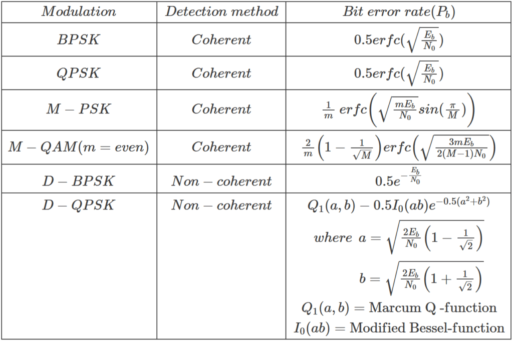
Table 1 summarizes the theoretical BER (given SNR per bit, the ratio – E_b/N₀) for various linear modulations. Note that the E_b/N₀ values used in that table are in linear scale [to convert E_b/N₀ in dB to linear scale – use E_b/N₀(linear) = 10^(E_b/N₀(dB)/10) ]. A small script written in Matlab (given below) gives the following output.

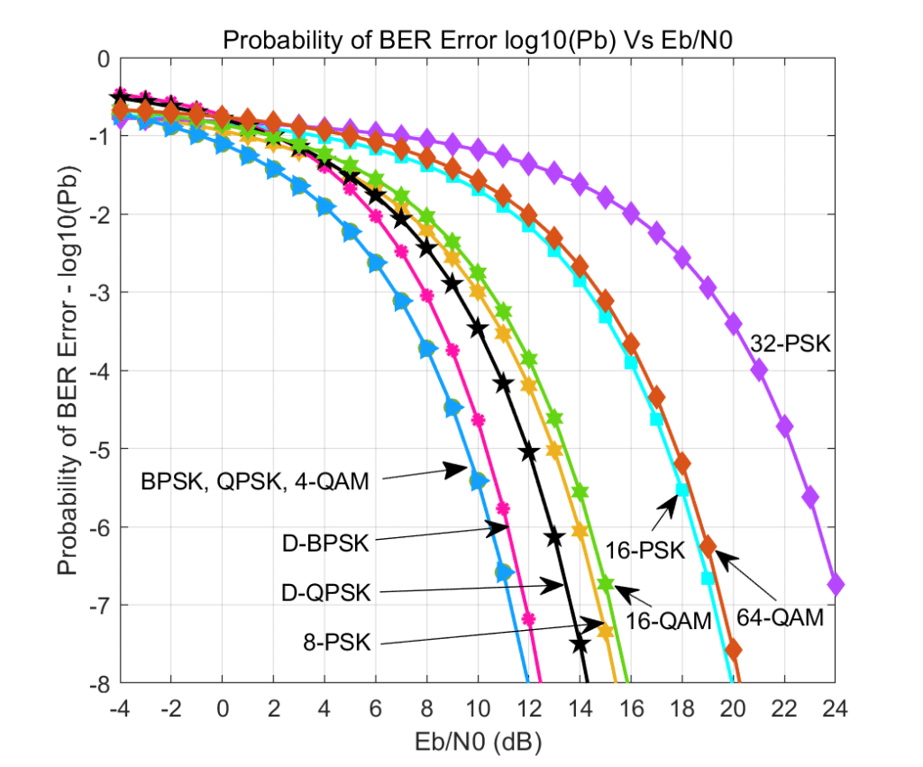
The following table is obtained by extracting the values of Eb/N0 to achieve BER=10^-6 from Figure-1. (Table data sorted with increasing values of E_b/N₀).

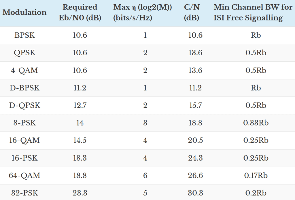
where,

\[\eta_B = \log_2 M \quad \text{bits/symbol}\]

is the bandwidth efficiency for linear modulation with M point constellation, meaning that η_B bits can be stuffed in one symbol with R_b bits/sec data rate for a given minimum bandwidth.

\[B_{\min} = \frac{R_b}{\eta_B}\]

is the minimum bandwidth needed for information rate of R_b bits/second. With raised-cosine pulse shaping of roll-off \(\alpha\), the two-sided passband occupancy becomes

\[B = (1+\alpha)\frac{R_b}{\eta_B}\]

Next the data in table 2 is plotted with E_b/N₀ on the x-axis and η on the y-axis (see figure 2) along with the well known Shannon’s Capacity equation over AWGN given by,

\[C = W \log_2\left(1 + \frac{C}{W}\frac{E_b}{N_0}\right)\]

The logarithm is base 2, because the next line inverts it with a power of two. Solving for \(E_b/N_0\) gives the Shannon curve drawn in Figure 2 (see Proakis, the reference below).

\[\frac{E_b}{N_0} = \frac{2^{C/W} – 1}{C/W}\]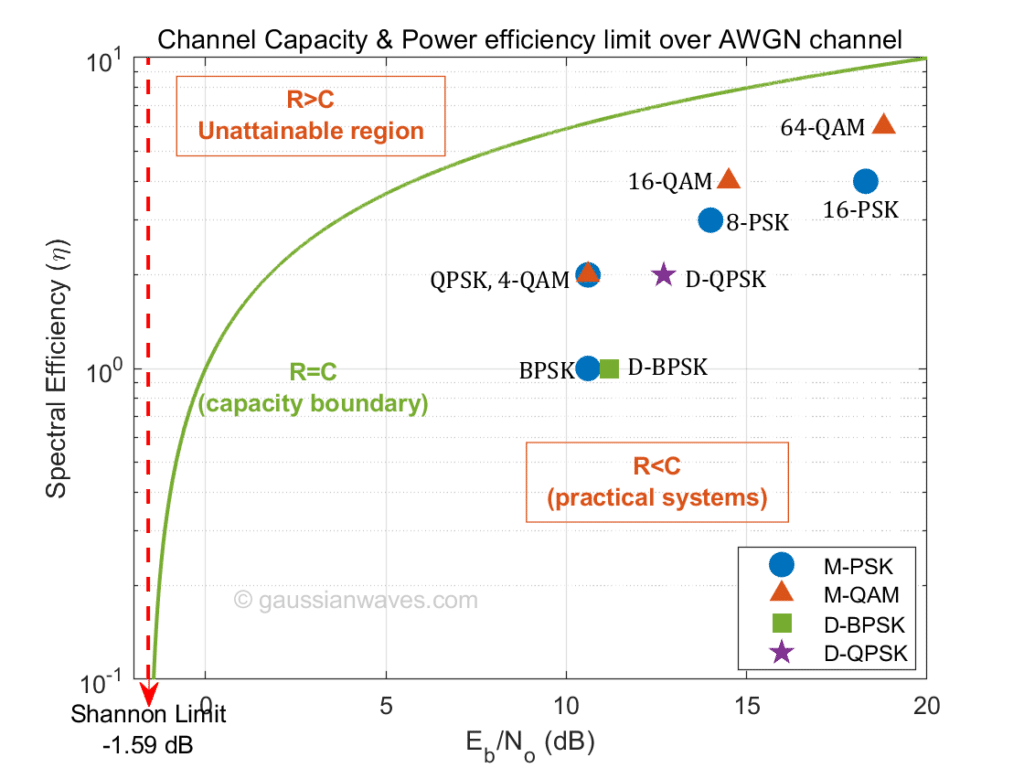

Matlab Code

EbN0dB=-4:1:24;
EbN0lin=10.^(EbN0dB/10);
colors={'b-*','g-o','r-h','c-s','m-d','y-*','k-p','b-->','g:<','r-.d'};
index=1;

%BPSK
BPSK = 0.5*erfc(sqrt(EbN0lin));
plotHandle=plot(EbN0dB,log10(BPSK),char(colors(index)));
set(plotHandle,'LineWidth',1.5);
hold on;

index=index+1;

%M-PSK
m=2:1:5;
M=2.^m;
for i=M,
    k=log2(i);
    berErr = 1/k*erfc(sqrt(EbN0lin*k)*sin(pi/i));
    plotHandle=plot(EbN0dB,log10(berErr),char(colors(index)));
    set(plotHandle,'LineWidth',1.5);
    index=index+1;
end

%Binary DPSK
Pb = 0.5*exp(-EbN0lin);
plotHandle = plot(EbN0dB,log10(Pb),char(colors(index)));
set(plotHandle,'LineWidth',1.5);
index=index+1;

%Differential QPSK
a=sqrt(2*EbN0lin*(1-sqrt(1/2)));
b=sqrt(2*EbN0lin*(1+sqrt(1/2)));
Pb = marcumq(a,b,1)-1/2.*besseli(0,a.*b).*exp(-1/2*(a.^2+b.^2));
plotHandle = plot(EbN0dB,log10(Pb),char(colors(index)));
set(plotHandle,'LineWidth',1.5);
index=index+1;

%M-QAM
m=2:2:6;
M=2.^m;

for i=M,
    k=log2(i);
    berErr = 2/k*(1-1/sqrt(i))*erfc(sqrt(3*EbN0lin*k/(2*(i-1))));
    plotHandle=plot(EbN0dB,log10(berErr),char(colors(index)));
    set(plotHandle,'LineWidth',1.5);
    index=index+1;
end

legend('BPSK','QPSK','8-PSK','16-PSK','32-PSK','D-BPSK','D-QPSK','4-QAM','16-QAM','64-QAM');
axis([-4 24 -8 0]);
set(gca,'XTick',-4:2:24); %re-name axis accordingly
ylabel('log10 of bit error rate');
xlabel('Eb/N0 (dB)');
title('Bit error rate against Eb/N0');
grid on;

FAQ

What is the recommended reading order? Follow the five lessons at the top: BPSK → QPSK → M-PSK → QAM → EVM. Use the BER and EVM calculators to check numbers as you go.

Similar articles

• 1. BPSK
• 2. QPSK
• 3. M-PSK sim
• 4. QAM sim
• 5. EVM
• Tool: BER vs Eb/N0 calculator
• Eb/N0, Es/N0 and SNR conversions

Reference

[1] “Digital Communications” by John G.Proakis , Chapter 7: Channel Capacity and Coding.↗

Related topics